Patterns of divergence and gene flow between populations and species

January 2016

Simon Martin ([email protected])

Introduction

In this practical we use genomic data from several populations of Heliconius butterflies to explore patterns of divergence and gene flow across a chromosome.

The hypotheses

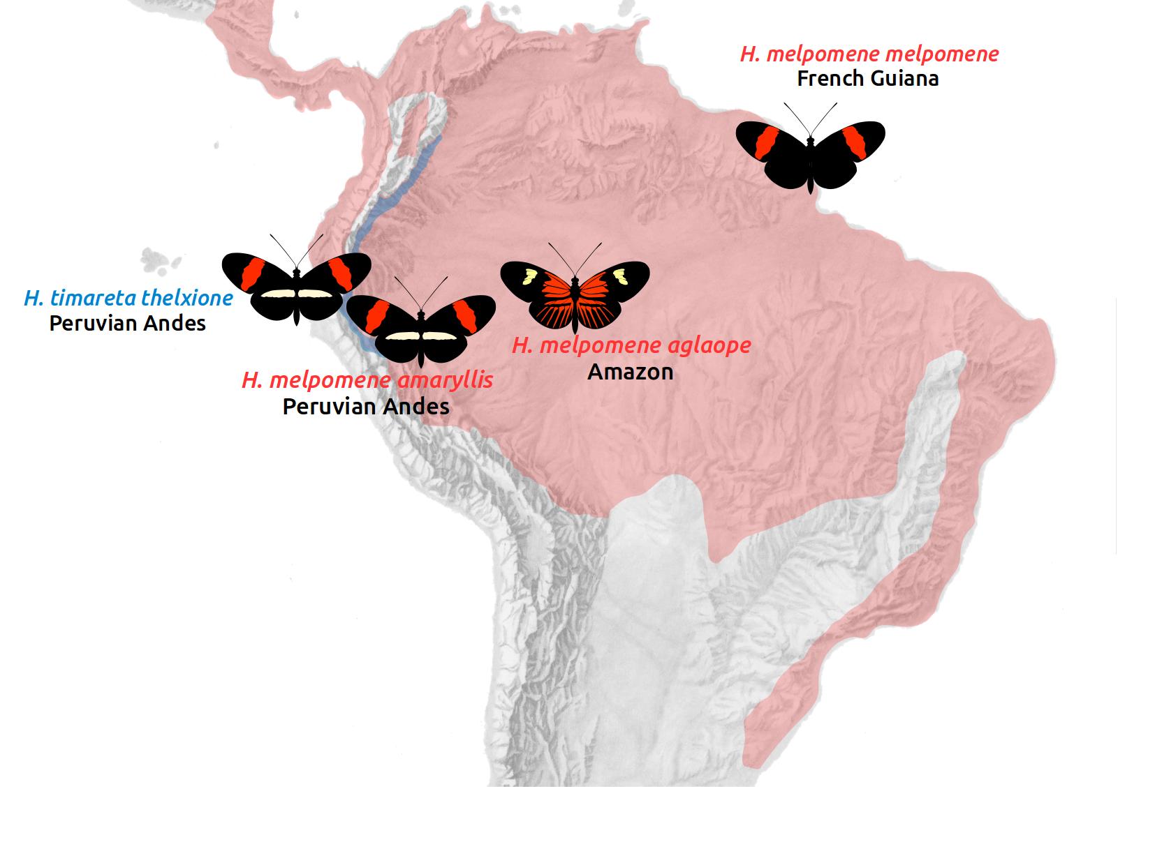
We will study four populations: three races of Heliconius melpomene and one race of its sibling species, Heliconius timareta. H. melpomene amaryllis occurs on the Andean slopes in Peru. H. m. aglaope ranges from the Andes into the Amazon basin. These two races are parapatric, with a narrow hybrid zone in Peru, where they mate freely. They have distinct wing patterns, which are controlled by two Mendelian loci on chromosomes 15 and 18. These distinct patterns are maintained in the face of random mating by strong divergent selection, so we predict that these loci should stand out as islands of elevated divergence against a largely undifferentiated background.

H. timareta occurs in sympatry with H. melpomene along the Andean slopes. The Peruvian race H. t. thelxinoe is sympatric with H. m. amaryllis, and the two have identical wing patterns. They differ in their ecology, and show strong assortative mating, although fertile hybrids can be produced. We predict generally elevated divergence between these populations, but there may also be evidence of gene flow.

We also include the completely allopatric race H. m. melpomene from French guiana. This serves to provide a baseline for patterns of divergence in the absence of gene flow.

The pipeline

We start with a VCF file with data from four samples from each population and one outgroup sample. The file includes 22 scaffolds representing chromosome 18 of the H. melpomene genome. We will filter and manipulate the VCF to produce two data files. The first will include all confident genotype calls, and will be used to study patterns of divergence between and diversity within populations (F_ST, d_XY and π). The second file will contain only variable sites, and will be used to estimate rates of gene flow between the two species using ABBA BABA statistics.

The VCF manipulation will be performed using bcftools (v. 1.2) and some command line hacking, and the subsequent analyses will be performed using Python and R. We will be using custom-written functions for all analyses.

General

To run this exercise, please connect to the AMI once again with ssh or PuTTY. You will find all input files in directory ~/wpsg_2016/activities/divergence-gene_flow. The R commands of the exercise can be executed either directly on the command line, or using Rstudio through a browser on your machine, by specifying http://YOUR_PUBLIC_DNS:8787 in the browser’s address bar.

Part 1 – Preparing inputs from VCF

The VCF file was produced by mapping whole genome Illumina data to the Heliconius melpomene genome using bwa mem and calling genotypes using GATK UnifiedGenotyper. The population VCFs were then merged and the 22 scaffolds of chromosome 18 were extracted using bcftools. The file has been compressed using bgzip, but can be read directly by bcftools.

Extracting all confident genotypes

First, we want to measure both divergence between and diversity within populations, so we will make a data file with both variant and invariant sites. The scripts we will use later take as input a tab-delimited file with columns for the chromosome (or scaffold), position and genotypes for each individual. These correspond to columns 1, 2 and 10-upwards in the VCF.

A quick way to make a header for our new data file is to extract just these fields from the VCF header:

bcftools view -h hel.18.vcf.gz | tail -1 | cut -f 1,2,10- > header.txt

Now we extract just the information we want from the VCF. Because this is a multi-step command, we will pipe to less each time to check that each part is working.

First, we remove all genotypes with depth (DP) < 10 or genotype quality (GQ) less than 30. Rather than discarding the entire line, we just set these to null genotypes (./.).

bcftools filter -e 'FORMAT/DP<10 | FORMAT/GQ<30' --set-GTs . hel.18.vcf.gz | less -S

Next we need to extract the scaffold, position and just the genotype for each sample. We use bcftools query and specify the fields %CHROM, %POS and %TGT, the latter meaning translated genotype (i.e., A/T as opposed to 0/1). We separate these with tabs (\t), and use [] to indicate that we want the genotype for all individuals. We also add a final filter to exclude all sites with fewer than 10 individuals (20 alleles) genotyped.

bcftools filter -e 'FORMAT/DP<10 | FORMAT/GQ<30' --set-GTs . hel.18.vcf.gz |
bcftools query -f '%CHROM\t%POS[\t%TGT]\n' -e 'AN < 20' | less -S

We want the genotypes encoded as AA, AT, NN, etc. for the scripts we will use later, so we use sed to remove the / and replace . with N.

bcftools filter -e 'FORMAT/DP<10 | FORMAT/GQ<30' --set-GTs . hel.18.vcf.gz |
 bcftools query -f '%CHROM\t%POS[\t%TGT]\n' -e 'AN < 20' |
 sed -e 's/\///g' -e 's/\./N/g' | less -S

Last, we cat the header file, gzip the result and send it to a new file.

bcftools filter -e 'FORMAT/DP<10 | FORMAT/GQ<30' --set-GTs . hel.18.vcf.gz |
 bcftools query -f '%CHROM\t%POS[\t%TGT]\n' -e 'AN < 20' |
 sed -e 's/\///g' -e 's/\./N/g' |
 cat header.txt - | gzip >  hel.18.DP10GQ30min10.geno.gz

Extracting only bi-allelic SNPs

For the ABBA BABA analysis, we only need to consider bi-allelic SNPs, so we will make a similar data file, but this time excluding all sites that don’t have exactly one alternate allele (N_ALT!=1) and where the minor allele is present less than twice (MAC<2).

bcftools filter -e 'FORMAT/DP<10 | FORMAT/GQ<30' --set-GTs . hel.18.vcf.gz |
 bcftools query -f '%CHROM\t%POS[\t%TGT]\n' -e 'N_ALT!=1 | AN<20 | MAC<2' |
 sed -e 's/\///g' -e 's/\./N/g' | cat header.txt - | gzip >  hel.18.DP10GQ30min10.BI.geno.gz

Part 2 – Diversity and divergence across the chromosome

Patterns of divergence across the genome can inform us about divergent selection and differential gene flow. Such studies typically use F_ST. However, the inability of this relative measure of divergence to differentiate between reduced inter-species migration and reduced intra-species diversity has prompted researchers to also consider absolute divergence (d_XY), and nucleotide diversity (π) within populations (e.g. Cruickshank and Hahn 2014).

Sliding window analysis in Python

We will calculate these measures across the chromosome in sliding windows. We will write a short Python script to do this. It will make use of several pre-written functions and classes for making the sliding windows and calculating the population genetic statistics.

An updated version of genomics.py should be first downloaded with wget and used to replace the original one, which has a bug.
Change to the exercise directory and download the new version of the script:
cd /home/ubuntu/wpsg_2016/activities/divergence-gene_flow
rm genomics.py
wget https://www.dropbox.com/sh/929dqzwjiynpcoz/AAA8nBXZSRIJhI8sv-yZMszua/genomics.py

Now, you can start writing the python script in your favorite text editor and test it with ipython similarly as in the python exercise.

First, we import the gzip library, so that we can read the zipped file directly. We also import all of the functions and classes in the genomics.py script provided.

import gzip
import genomics

Define the input file and create a file handle.

genoFileName = "hel.18.DP10GQ30min10.geno.gz"
genoFile = gzip.open(genoFileName, "r")

Provide names for the populations in our dataset, and list the individuals in each.

We have three H. melpomene populations:

amaryllis (“ama”) from Peru
aglaope (“agl”) from Peru
melpomene (“melG”) from Guiana

One H. timareta population:

thelxinoe (“thxn”) from Peru

And an outgroup:

H. pardalinus sergestus (“ser”)

popNames = ["ama","agl","melG","thxn","ser"]

samples = [["ama.JM160","ama.JM216","ama.JM293","ama.JM48"],
           ["agl.JM108","agl.JM112","agl.JM569","agl.JM572"],
           ["melG.CJ13435","melG.CJ9315","melG.CJ9316","melG.CJ9317"],
           ["thxn.JM313","thxn.JM57","thxn.JM84","thxn.JM86"],
           ["ser.JM202"]]

Create a sampleData object, which stores this population information.

sampleData = genomics.SampleData(popInds = samples, popNames = popNames)

Set the run parameters. We will use a window of 50 kb, a step size of 25 kb, and we will set a minimum number of genotyped sites per window to 25,000. Note that these windows are based on genomic coordinates, so each window always represents a 50 kb region of the genome, even if the number of genotyped sites within that region is much smaller. An alternative approach would be to use a fixed number of SNPs within each window, but then each window might represent a different sized region of the genome.

windSize = 50000
stepSize = 25000
minSites = 25000

Now we create a windowGenerator object. This is a custom-written function that simply reads the input file and passes us one window of genotype data at a time. It will check that no window is greater than the defined size, and that windows do not overlap scaffold boundaries. It is a Python generator object, which means it does not create all the windows at once but only creates a new window when requested.

windowGenerator = genomics.slidingWindows(genoFile, windSize, stepSize, skipDeepcopy = True)

Define and open the output file.

outFileName = "pop_div.w50m25s25.csv"
outFile = open(outFileName, "w")

Write the header line for the output file, which will include “pi” for each population, and “Fst” and “dxy” for each pair of populations.

outFile.write("scaffold,start,end,sites")

for x in range(len(popNames)-1):
    outFile.write(",pi_" + popNames[x])
    for y in range(x+1,len(popNames)):
        outFile.write(",Fst_" + popNames[x] + "_" + popNames[y])
        outFile.write(",dxy_" + popNames[x] + "_" + popNames[y])

outFile.write("\n")

Now we run the sliding window analysis. For each window we start by checking that there are enough sites in the window. If so, we make an Alignment object and calculate F_ST, d_XY and π using the function genomics.popDiv. We collect the results as well as window information (scaffold, start, end and number of sites) and then write to the output file.

n=0
for window in windowGenerator:
    if window.seqLen() >= minSites:
        #if there are enough sites, make alignment object
        Aln = genomics.callsToAlignment(window.seqDict(), sampleData, seqType = "pairs")
        #get divergence stats
        statsDict = genomics.popDiv(Aln)
        stats = []
        for x in range(len(popNames)-1):
            #retrieve pi for each population
            stats.append(statsDict["pi_" + popNames[x]])
            for y in range(x+1,len(popNames)):
                #retrieve dxy and Fst for each pair
                stats.append(statsDict["fst_" + popNames[x] + "_" + popNames[y]])
                stats.append(statsDict["dxy_" + popNames[x] + "_" + popNames[y]])
        #add window stats and write to file
        out_data = [window.scaffold, window.start, window.end, window.seqLen()] + [round(s,3) for s in stats]
        outFile.write(",".join([str(x) for x in out_data]) + "\n")
    print n
    n+=1

Close files and exit.

outFile.close()
genoFile.close()


exit()

Plotting results in R

Read the data file into R.

div_data <- read.csv("pop_div.w50m25s25.csv", as.is=T)

Define position as the midpoint between window start and end.

div_data$position <- (div_data$start + div_data$end)/2

The positions are still with respect to scaffold. We can convert these to chromosome positions by adding the scaffold offset for each scaffold. To do this, we need to read in the provided file of scaffold positions. We read the first column (scaffold) as row names, which will allow us to index by scaffold.

scaf_positions <- read.csv("chr18_scaffold_positions.csv", row.names = 1)

We can then make a vector of offsets (scaffold start points) for each window in our dataset. By adding window position to this offset we get chromosome position for each window.

scaf_offset <- scaf_positions[div_data$scaffold, 1]
div_data$chrom_pos <- div_data$position + scaf_offset

As we will be making multiple plots, we can write a simple function to plot the data across the chromosome. This will take several variable names as Y variables and specified colours for each.

chromosome_plot <- function(dataframe, Xname, Ynames, cols, xlim, ylim, ylab){
    plot(0,xlim=xlim,ylim=ylim,cex=0,ylab=ylab,xlab="Position")
    for (y in 1:length(Ynames)){lines(dataframe[,Xname], dataframe[,Ynames[y]], type = "l", col = cols[y])}
    legend(xlim[2]/2, ylim[2], legend = Ynames, lty = 1, col = cols, bty = "n", ncol = 2)
    }

Here is an example of two F_ST plots. The first shows F_ST between races of H. melpomene (parapatric and allopatric), and the second shows F_ST between H. melpomene and H. timareta in sympatry vs allopatry.

par(mfrow = c(2,1), mar = c(4,4,1,1))

chromosome_plot(div_data, "chrom_pos", c("Fst_ama_agl", "Fst_ama_melG"),
                c("red","blue"), xlim =c(0,17000000), ylim =c(0,1), ylab = "Fst")

chromosome_plot(div_data, "chrom_pos", c("Fst_ama_thxn", "Fst_melG_thxn"),
                c("forest green","violet"), xlim = c(0,17000000), ylim = c(0,1), ylab = "Fst")

Exercise:

Make plots to explore the following questions:

How do patterns of divergence differ between races and species, in sympatry and allopatry? (Note, the wing patterning locus is at around 1 – 1.5 Mb.
Do peaks of F_ST tend to represent peaks of absolute divergence or troughs in diversity?

If there’s time…

How does changing the window size and step size affect the results?

Part 3 – Estimating rates of gene flow across the chromosome

We will now use a more direct method to explore how rates of gene flow differ across the chromosome. The ABBA BABA statistics are used to detect and quantify an excess of shared derived alleles, which can be indicative of gene flow. Given three populations and an outgroup with the relationship (((P1, P2),P3) O), these statistics test for sharing of genetic variation between P3 and P2 but not with P1. The choice of P1 can therefore affect the results, as we shall see.

We will consider two simple statistics: D (Green et al. 2010, Durand et al. 2011) simply compares the counts of shared derived alleles between P2 and P3, wheras f_d (Martin, Davey and Jiggins 2015) attempts to control for some of the biases of D, and is more suitable for sliding windows.

Sliding window analysis in Python (again)

We will once again calculate these measures in sliding windows, using a Python script very similar to that used above.

To begin, we will follow the same steps as in Part 2 to load the necessary libraries, open the input file (except here we use the SNPs-only file hel.18.DP10GQ30min10.BI.geno.gz) and define the populations and samples.

We now have to specify the populations for the ABBA BABA test. First, we want to test for sharing of wing patterning alleles between H. t. thelxinoe and H. m. amaryllis but not with its parapatric partner H. m. aglaope. So we make the latter P1.

P1 = "agl"
P2 = "ama"
P3 = "thxn"
O = "ser"

We need to make an output file specifically for this test, and write a header line including columns for the two statistics: D and f_d.

outFileName = "ABBA_BABA_agl_ama_thxn_ser.w50m1s25.csv"
outFile = open(outFileName, "w")

outFile.write("scaffold,start,end,sites,ABBA,BABA,D,fd\n")

Then define the window parameters and make a windowGenerator object as in Part 2. We are now using only bi-allelic SNPs, so the minimum sites should be reduced to around 1000 per 50 Kb window.

The loop that analyzes each window is similar to above, except here we use a function called genomics.ABBABABA to generate the statistics.

n=0
for window in windowGenerator:
    if window.seqLen() >= minSites:
        #make alignment object
        Aln = genomics.callsToAlignment(window.seqDict(), sampleData, seqType = "pairs")
        #get ABBA BABA stats
        statsDict = genomics.ABBABABA(Aln, P1, P2, P3, O)
        stats = [statsDict[s] for s in ["ABBA","BABA","D","fd"]]
        #add window stats and write to file
        out_data = [window.scaffold, window.start, window.end, window.seqLen()] + [round(s,3) for s in stats]
        outFile.write(",".join([str(x) for x in out_data]) + "\n")
    print n
    n+=1

To estimate rates of gene flow over the whole chromosome, repeat this procedure, but using the allopatric H. m. melpomene from French Guiana (“melG”) as P1. Remember to change the name of the output file.

Plotting

We can use similar R plotting code to that in Part 2 to create plots of D and f_d across the chromosome. Note that D ranges from -1 to 1 and f_d from 0 to 1.

Exercise

How does the identity of P1 affect measures of gene flow?
Which regions show evidence of introgression between species?

Divergence and gene flow exercise