
Probability in evolutionary genomics
Milan Malinsky, 06 June 2022
Background and Objectives
Thinking about probabilities is one of cornerstones of population and speciation genomics. We often aim to evaluate the strength of evidence for a particular conclusion and quantify the uncertainties associated with it. We also often want to estimate parameters of evolutionary models, e.g, of populations. In this exercise, we are going to explore a number of examples of probabilities in (evolutionary) genomics.
Learning goals:
- Get familiar with probabilities and likelihood in the context of genomics
- Appreciate base calling errors, finite sampling of reads from diploid individuals, and finite sampling of individuals from populations as sources of uncertainty
- Recognise the Binomial distribution and where it applies
- Use R code to explore these questions and plot the results
- Consider how appreciation of probabilities may affect you experimental choices and interpretation in the context of estimating FST
Table of contents
Most genomic data analyses start with DNA reads. You are probably familiar with output of a DNA sequencer in the standard FASTQ format. Here is one DNA read (150bp):
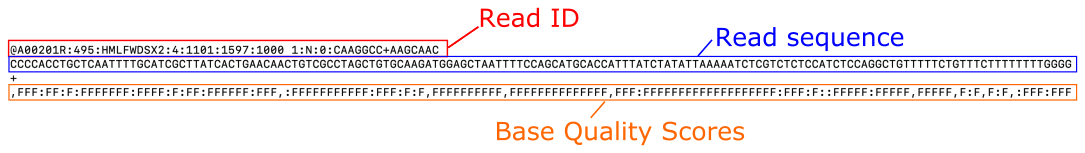
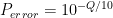
The base qualities output by the sequencing machine are encoded so that each character corresponds to a number (a score). For example , = 11, : = 25, and F = 37. The full translation list can be found for example on this Illumina webpage. The quality scores in turn correspond to base calling error probabilities, such, that if we denote the score as 

,:F,F?
Show me the answer!
- The quality scores corresponding to the sequence of five characters
,:F,Fare 11, 25, 37, 11, and 37. - The probabilities corresponding to those quality scores are: 0.0794, 0.0031, 0.0002, 0.0794, and 0.0002
- The expected number of errors is: 0.0794 + 0.0031 + 0.0002 + 0.0794 + 0.0002 = 0.16
Show me the answer!
 in each trial. Those of you with some background in statistics will recognise that the total number of failures (base calling errors), let’s denote it by
  , has the Binomial distribution. In mathematical notation:
  .
.
To answer our question, we can then use the Binomial Cumulative Distribution Function, for example as implemented in R:
- The probability of seeing at least one error:
pbinom(0, 150, 0.01,lower.tail=FALSE) - The probability of seeing at least two errors:
pbinom(1, 150, 0.01,lower.tail=FALSE) - The probability of seeing at least three errors:
pbinom(2, 150, 0.01,lower.tail=FALSE)
As you can see in the R output, the probabilities are approximately 78%, 44% and 19%.
Show me the answer!
We can calculate this easily from the results above. The probability of seeing exactly two sequencing errors is the probability of seeing at two or more errors minus the probability of seeing exactly three or more errors. So, approximately 44% – 19% = 25%.
Translated to R code: pbinom(1, 150, 0.01,lower.tail=FALSE) - pbinom(2, 150, 0.01,lower.tail=FALSE)
Alternatively we can answer this question directly, using the R implementation of the Binomial Probability Mass Function: dbinom(2, 150, 0.01)
Most of us study diploid organisms. This means that when we sequence DNA of an individual, the reads come as a random mixture of the two homologous chromosomes. The presence of heterozygous sites, i.e. loci where the two homologous chromosomes differ, presents a statistical challenge when estimating genotypes. This is true for the majority of the genome, except for mitochondrial DNA and sex chromosomes.
Consider a biallelic locus and let the reference allele be represented as 0 and the alternative allele as 1. The possible diploid genotypes are then the homozygous 0/0 and 1/1, and the heterozygous 0/1.
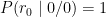
First, let us consider a scenario where, at a particular locus in the genome, we have one perfect read carrying the 0 allele. For now, we are going to simplify our lives and ignore base calling errors, (unrealistically) assuming that reads are perfect. We are also going to assume (again unrealistically), that we can place/map all the reads unambiguously to their matching place in the reference genome.
0 allele) given the genotypes?
Show me the answer!
- The probability of a read carrying the
0allele, denoted, given the homozygous
0/0genotype is: - The probability of a read carrying the
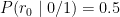
0allele, denoted0/1genotype is: - The probability of a read carrying the
0allele, denoted1/1genotype is:

These are the likelihoods, i.e.: 


In the above example, the 0/0 genotype has the highest likelihood, and, therefore, 0/0 is the maximum likelihood estimate of the genotype. However, notice that we cannot be certain that 0/0 is the correct genotype because there is a possibility that the read with the 0 allele originated from a heterozygous 0/1 locus. The Genotype Quality (GQ) field in a VCF file typically represents difference in between the most likely and the second most likely genotype (e.g. see details for GQ in GATK output).


GQ for this ‘single perfect read’ example?
Show me the answer!
- In numbers:
- In R code:
GQ = -10*log10(0.5) - (-10*log10(1))

In the VCF file, the number is rounded to the nearest integer to save space. So GQ = 3 for the 0/0 call.
It is common practice (although probably not the best practice) to filter variants based on GQ and set genotypes with GQ falling below a particular threshold to missing. This threshold is often set to keep variants with GQ >=20.
0/0, how many reads (how much read depth) do we need to call the 0/0 genotype with GQ >= 20?
Show me the answer!
As we increase the read depth, all additional reads are going to carry the 0 allele, because the true genotype is 0/0 and the reads have no base-calling errors. Therefore, the likelihood of the (correct) 0/0 genotype is going to always remain 1. However, as we add more reads (evidence), the likelihood of the (erroneous) 0/1 genotype is going to decrease. We need it to decrease sufficiently that its 
; therefore, we require the likelihood of the
0/1genotype to decrease below 0.01.
Let’s remind ourselves that the likelihood of the 0/1 genotype is the probability of seeing the read(s), given this genotype. If the 0/1 genotype were correct, any read would have 50% probability of carrying the 0 allele and 50% probability of carrying the 1 allele. The probability of seeing one read carrying the 0 allele is then 
0 allele is 
0 allele is 


GQ >= 20.
3) Genome coverage distributions
The GQ >= 20 threshold corresponds to getting about one in 100 genotype calls wrong, which may seem acceptable, and the above example suggests that about 7 perfect reads are needed to make a genotype call with this confidence in a diploid individual. We might therefore be tempted to sequence our individuals to 7x genome coverage. However, we should remember that while this would be the average coverage any particular site might be covered by more reads, or fewer reads.
If we assume that each read has an equal chance of coming from anywhere in the genome (which is not quite true, but close enough in whole genome sequencing; see e.g. this paper), the coverage at any one site (let’s denote it 
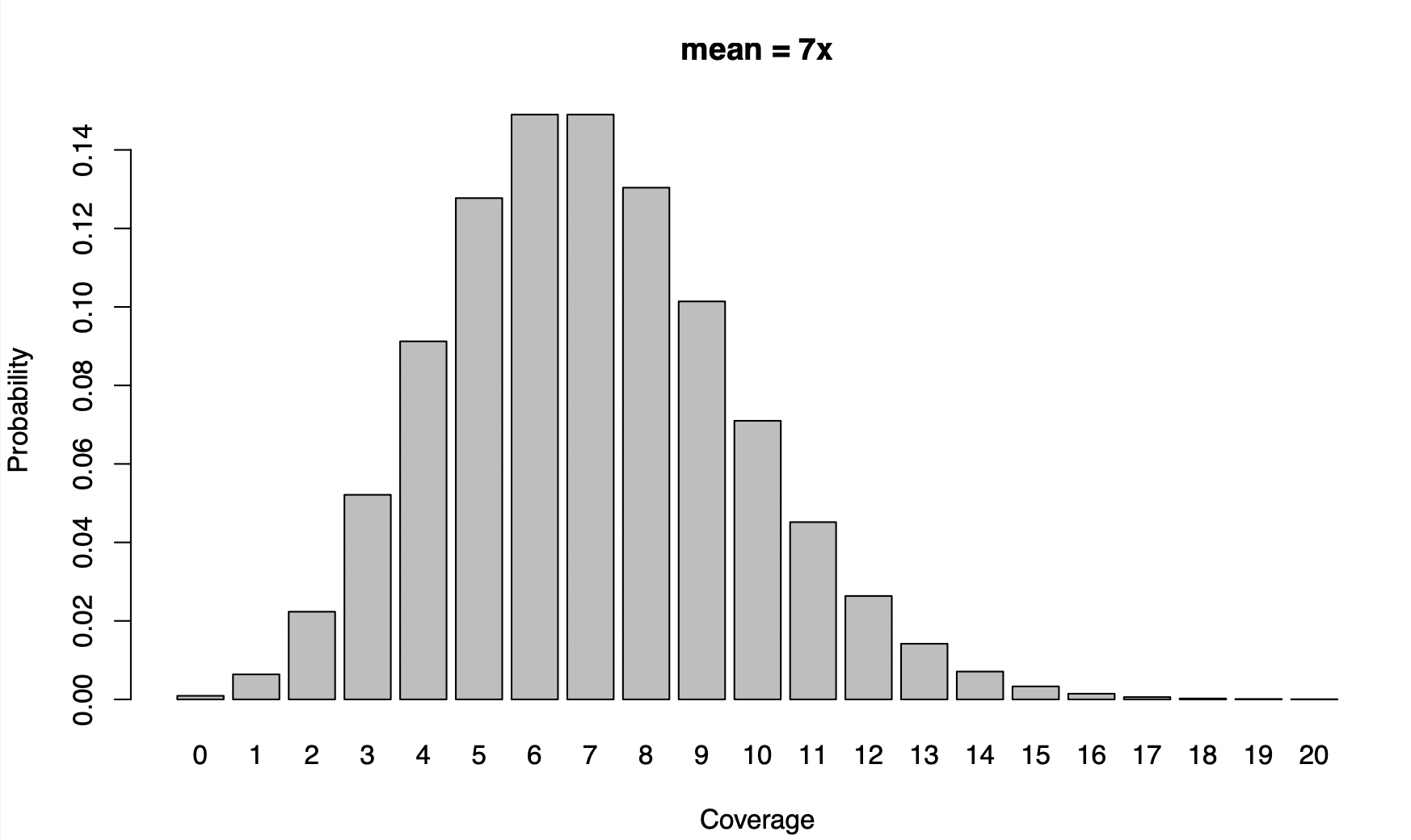
Code: barplot(dpois(0:20,7),names=0:20, main="mean = 7x",xlab="Coverage",ylab="Probability")
dpois() and the Cumulative Density Function is ppois(). Can you use R to find the proportion of sites with less than 7x coverage? How about less than 3x coverage?
Show me the answer!
For the first question, 
; Both
sum(dpois(0:6,7))andppois(6,7,lower.tail=T)provide this answer; The R code:
sum(dpois(0:2,7))orppois(2,7,lower.tail=T)
Show me the answer!
With 
; The R code:
sum(dpois(0:6,10))orppois(6,10,lower.tail=T); The R code:
sum(dpois(0:2,10))orppois(2,10,lower.tail=T)
As you can see, a modest increase in mean coverage (from 7 to 10x) results in proportionally much greater decrease in sites having low coverage (below 7x or 3x).
Show me the answer!
To answer this question, we can plot 
The R code:
plot(10:20,ppois(6,10:20,lower.tail=T),xlab="Mean coverage",ylab="P(X < 7)")
abline(h=0.01,col="red")
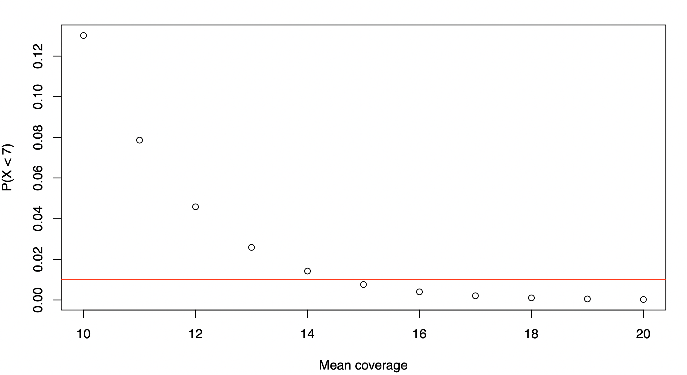
We can see that the proportion of sites with coverage below 7x falls below 1% when the mean genome-wide coverage is increased to 15x.
4) Estimating FST (Associated R code)
There can be some ambiguity in usage of the term FST – not all people mean the same thing by FST. One can talk of FST as an evolutionary parameter; in this case, the same evolutionary parameter can give rise to different allele frequencies. We also talk of FST as a deterministic summary of allele frequencies. These summaries are designed to be estimators of the evolutionary parameter, but sometimes we refer to them simply as FST. In this exercise, we are going to use the Hudson estimator of FST, as defined in equation (10) of this paper, which also describes other estimators and discusses many practical choices involved in applying the estimates to modern genomic data.
FST estimators are a function of allele frequencies in a population or in multiple populations. A common use case in modern population and speciation genomic studies is to calculate pairwise FST estimates to assess differentiation between two populations at different loci along the genome. The pairwise Hudson FST estimator is:
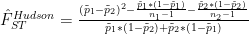
where 


In the following exercises, we are going to explore how the finite sampling of individuals affects estimates of allele frequencies and, how this, in turn, affects FST estimates. At this stage, we are going to ignore base and genotype calling uncertainties and assume we have perfect genotype calls. This allows us to explore directly the effect of the number of individuals in our sample.
We start by focussing on allele frequency estimates. Consider a biallelic SNP with a minor allele frequency (the frequency of the less common allele) of 0.45. In other words, 45% of the individuals in the population have the less common allele, e.g. an A and the remaining 55% of individuals have the more common (major) allele, e.g., a T.
Show me the answer!
Perhaps unsurprisingly, the Binomial distribution again provides an answer. If we encode the major allele as 0 and the minor allele as 1, then the probability of each observation of the minor allele in our sample is 0.45. Each observation is a Bernoulli trial and 0.45 is the probability of success (observing the minor allele). The number of minor alleles in our sample, let's denote it by 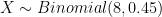


R code:
plot((0:8)/8,dbinom(0:8, size = 8, prob=0.45),pch=16,col="red",xlab="Sample allele frequency",ylab="Probability",cex=1.2,type='b',main="Population allele frequency = 0.45")
points((0:20)/20,dbinom(0:20, size = 20, prob=0.45),pch=16,col="blue",cex=1.2,type='b')
points((0:40)/40,dbinom(0:40, size = 40, prob=0.45),pch=16,col="orange",type='b',cex=1.2)
legend("topright",legend=c("4 diploid individuals","10 diploid individuals", "20 diploid individuals"),pch=16,col=c("red","blue","orange"))
We can see that the distributions have rather large variances. With four individuals, there is 31% probability that our sample allele frequency is going to be less than 0.25 or more than 0.75, very far from the true population allele frequency of 0.45: sum(dbinom(c(0,1,2,6,7,8), size = 8, prob=0.45)). This probability drops to 6% with ten diploid individuals (sum(dbinom(c(1:5,15:20), size = 20, prob=0.45))), and 0.7% with 20 diploid individuals (sum(dbinom(c(1:10,30:40), size = 40, prob=0.45))). Nevertheless, the uncertainty in these allele frequency estimates is considerable.


Show me the answer!
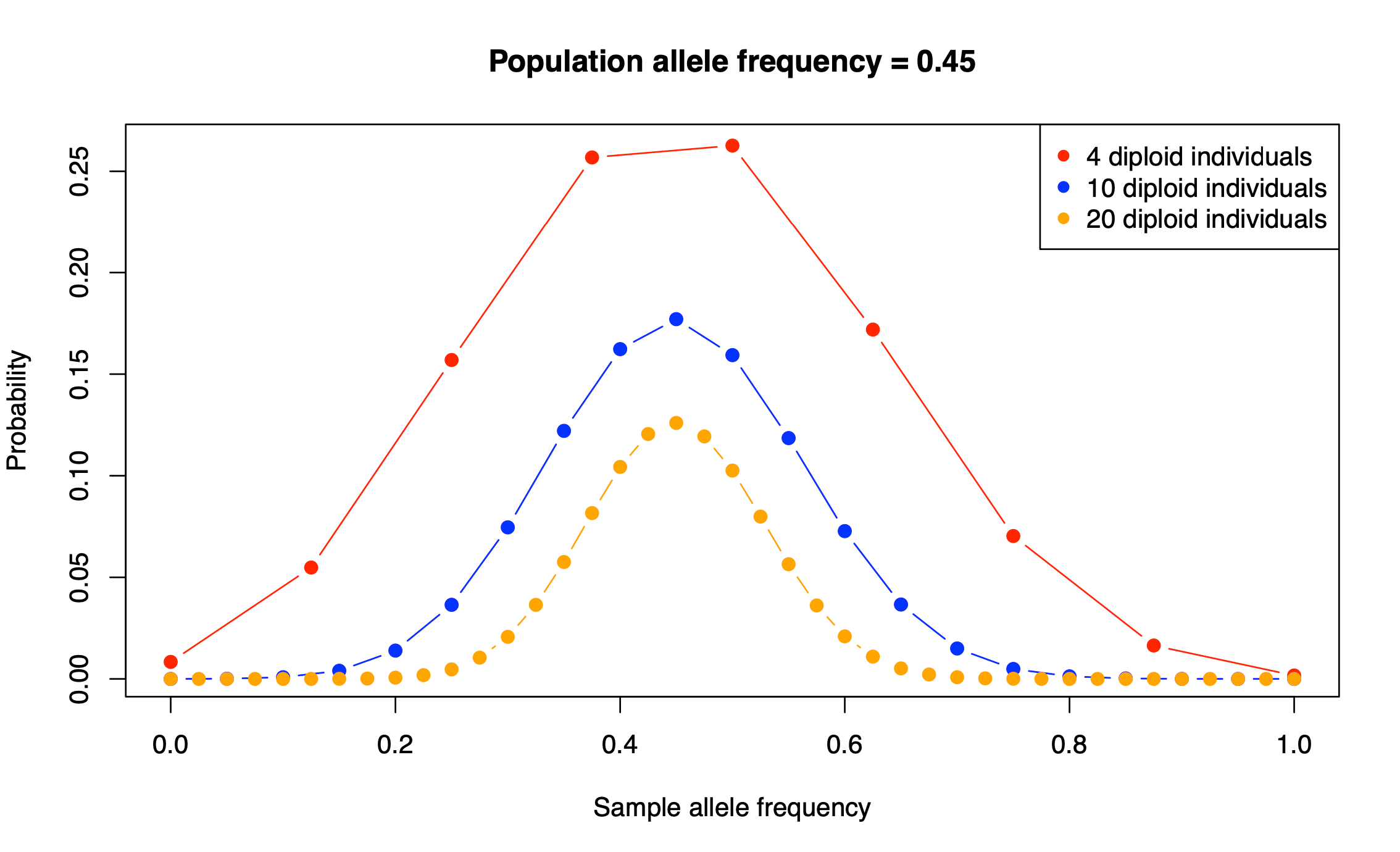
The distributions have become narrower. There is a better chance to obtain a more accurate estimate of this minor allele frequency. In fact, it is straightforward to formally show that it is indeed true. The variance of a random variable with a Binomial distribution is ![Var[X] = n*p*(1-p)](http://s0.wp.com/latex.php?latex=Var%5BX%5D+%3D+n%2Ap%2A%281-p%29&bg=ffffff&fg=000&s=0&c=20201002)


Let's say that a polymorphism has minor allele frequency of 0.45 in population 1 and 0.15 in population 2. The Hudson estimator returns FST = 0.194. Next we are going to explore how the uncertainties in allele frequency estimation translate into pairwise FST estimates for a single SNP.
Using R, we have drawn 100000 observations from the sample allele frequency distributions with 4, 10, and 20 diploid individuals from each of the two populations. Using these observations, we obtain the following FST values.

Is becomes apparent that the FST estimates with four diploid individuals are all over the place. In fact it is not much better with 10 diploid individuals. Only with 20 individuals we start getting a distribution that appears centred around the true population FST of 0.194 (this value is denoted by the red vertical lines in the plots above).
The variances are huge. However, it is not the case that the Hudson estimator does not work. On average, we are getting the right answer, or at least very close to it (there is slight underestimation). As indicated in the figure, the mean of the observations was around 0.18, reasonably close to 0.194, in all analyses, whether with 4, 10, or 20 individuals.
The fact that on average we get (almost) the right answer is the reason why genome scans for differentiation usually average over multiple SNPs.
Let's explore what happens to the variance of the FST estimator if we average over five, ten, or twenty independent SNPs. You can execute the provided R code and make your own plots, or click on the expanding boxes below.
See the results for five SNPs
The allele frequencies are for which we show results below are:
p1 = 0.375,0.018,0.159,0.273,0.064
p2 = 0.393,0.308,0.188,0.278,0.49
(you could use also use R to simulate five random minor allele frequencies: round(runif(5,max=0.5),3)
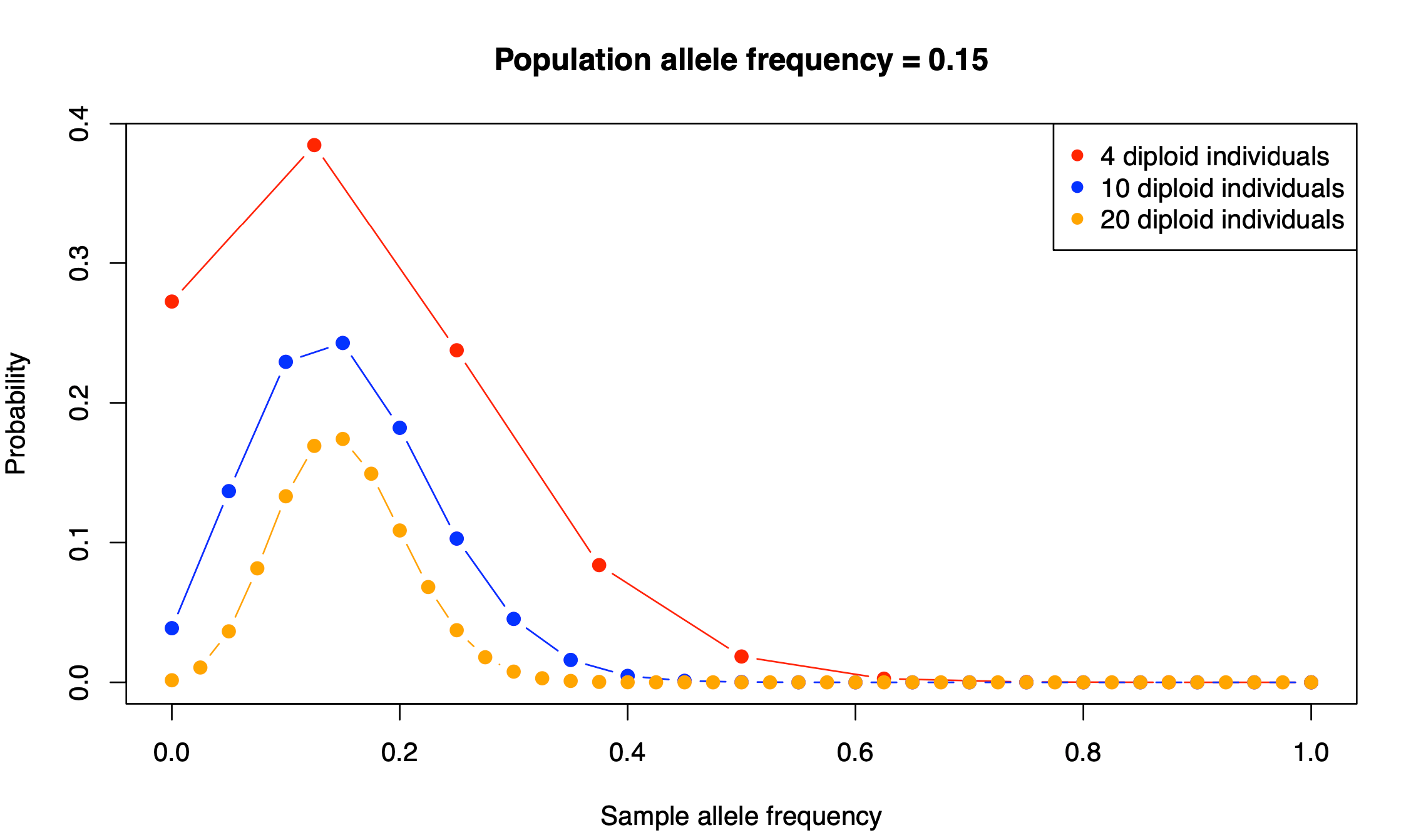
The population Hudson FST estimate for our p1 and p2 is 0.136. The distributions of FST estimates from sample allele frequencies with 4, 10, and 20 diploid individuals are shown below:
Compared with per-SNP estimates, the distributions based on 5 SNP averages have considerably lower variances. In particular, estimation based on sampling ten diploid individuals is starting to look possible.
See the results for ten SNPs
The allele frequencies are for which we show results below are:
p1 = 0.421,0.154,0.055,0.197,0.062,0.043,0.094,0.343,0.314,0.024
p2 = 0.03,0.423,0.052,0.407,0.157,0.038,0.285,0.4,0.172,0.352
The population Hudson FST estimate is 0.138, similar as in the five SNP case. Again, the distributions of FST estimates from sample allele frequencies with 4, 10, and 20 diploid individuals are shown below:
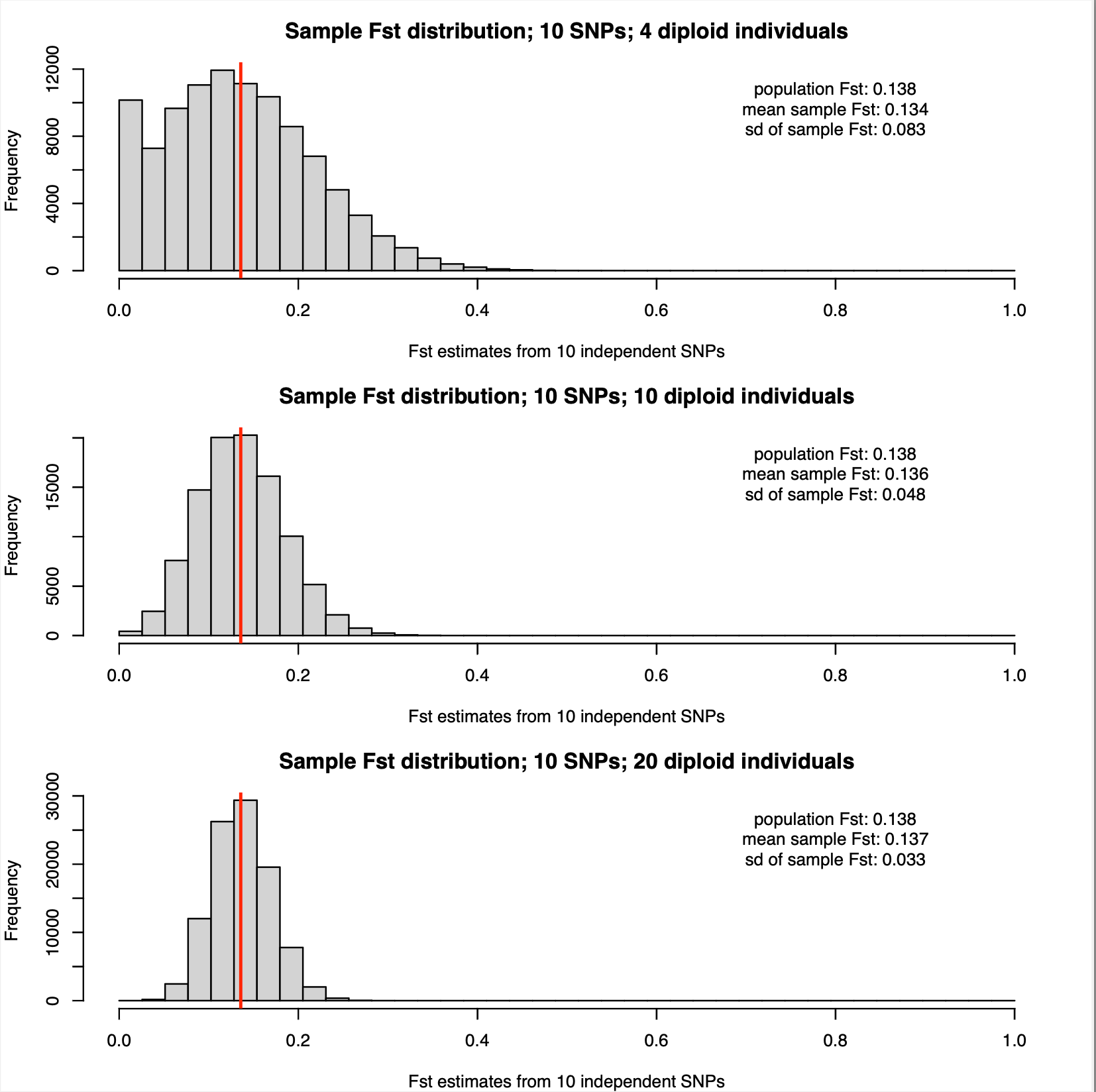
As expected the sampling distributions narrow further with 10 SNPs. However, relying on sampling four individuals from each population still seems like a bad idea for this estimation.
See the results for 20 SNPs
The allele frequencies are for which we show results below are:
p1 = 0.421, 0.154, 0.055, 0.197, 0.062, 0.043, 0.094, 0.343, 0.314, 0.024, 0.35, 0.344, 0.076, 0.406, 0.325, 0.369, 0.413, 0.033, 0.242, 0.027
p2 = 0.03, 0.423, 0.052, 0.407, 0.157, 0.038, 0.285, 0.4, 0.172, 0.352,0.013, 0.300, 0.200, 0.095, 0.425, 0.104, 0.154, 0.365, 0.184, 0.060
The population Hudson FST estimate is 0.138, again very similar similar as in the five and ten SNP cases.
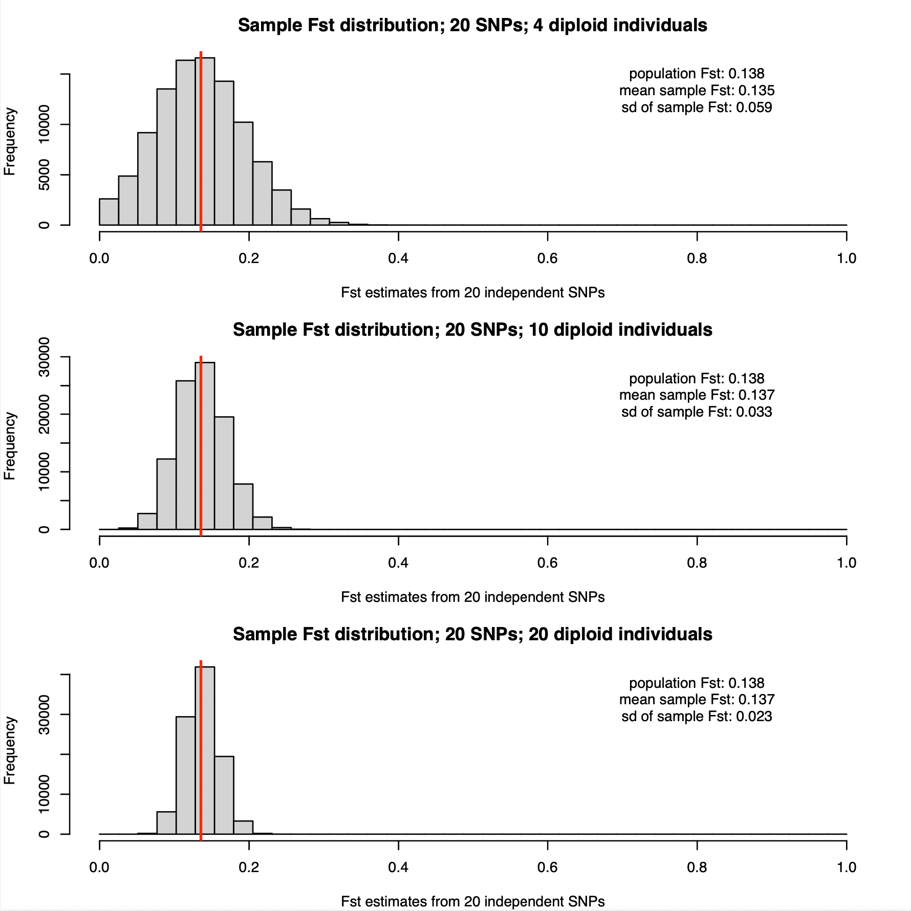
The sampling distributions narrow even further with 20 SNPs. Even using only 4 diploid individuals is starting to look reasonable with this window size. And with 20 diploid individuals, we are getting very accurate FST estimates, with standard deviation of only 0.02.
It can be overwhelming to try to compare all the above results. Luckily, because the mean population FST value was very similar in the above examples, it makes sense to overlay the inferred probability density plots to see all the results at a glance in a single plot.
See the density overlay of results for different window sizes

In this activity, you have explored a number of simple statistical concepts, such as probabilities, likelihood, probability distributions (Binomial, Poisson), and distribution functions in the context of evolutionary genomics. You have also seen how you can gain information about probabilities using a number of simple, but powerful functions implemented in the R environment for statistical computing. Such insights can inform your experimental design choices (e.g., sequencing instrument, depth of coverage, number of individuals sequenced from each population), and they can also help you to evaluate the strength of evidence provided by your data.
Having explored base calling error rates, finite read sampling, and finite sampling of individuals, you might be wondering how to combine these sources of uncertainty into a unified framework. This is indeed possible, and the math is not so complicated, although it is beyond the scope of this introductory exercise.
However, tomorrow you are going to learn about the program ANGSD, which performs population genetics analyses, including FST estimation and much more, while integrating over the sources of uncertainty arising from base calling error probabilities and from DNA read sampling.