
Species-tree inference with BEAST 2 and SNAPP
Michael Matschiner, 28 January 2020
Background and Aim
When estimating the species tree for a group of recently diverged species, there are multiple reasons to do so on the basis of the multi-species coalescent model. First, this model allows taking into account incomplete lineage sorting, which has been shown to improve the accuracy of both species-tree topology and branch lengths (Ogilvie et al. 2017). Second, by integrating incomplete lineage sorting, the multi-species coalescent model also allows the estimation of the population size. The multi-species coalescent model is implemented in a number of programs that can be used with different types of input data. Some programs, like StarBEAST (Ogilvie et al. 2017) or BPP (Yang 2015) expect multiple-sequence alignments from which they jointly estimate gene trees (= the genealogies of individual alignments) and the species tree.
Other programs like ASTRAL (Zhang et al. 2018) demand sets of gene trees as input; thus, to run these programs, gene trees must first be estimated with other tools. By eschewing gene-tree estimation, programs like ASTRAL are much faster than other implementations of the multi-species coalescent and can be applied to much larger datasets, but it is usually difficult to assess to what extend their species-tree estimate may be affected by incorrectly estimated gene trees.
A small number of programs (Bryant et al. 2012; Chifman and Kubatko 2014) also allows the estimation of species trees directly from SNP data, allowing in principle a different genealogy at each individual SNP. One advantage of this type of inference is that it can not be affected by within-locus recombination, given that each locus is only a single SNP. A second advantage is convenience, since genomic datasets usually come in variant call format and would be difficult to convert to sequence alignments. On the other hand, estimating individual genealogies for each SNP would be extremely computationally demanding and each of these genealogies would have extremely low resolution, given that only few states can be observed per SNP. To avoid this issue, the Bayesian program SNAPP (SNP and AFLP Package for Phylogenetic analysis; Bryant et al. 2012), available as an add-on package for BEAST 2 (Bouckaert et al. 2019), does not estimate the genealogies of all SNPs but instead integrates over all possible genealogies at each SNP mathematically. This approach is still very computationally demanding, but makes the analysis feasible at least for datasets of thousands of SNPs and around 10-20 species (Stange et al. 2018).
Learning goals
- Familiarize yourself with Bayesian analyses using the BEAST 2 suite of programs.
- Learn how to estimate the species tree from SNP data with the multi-species coalescent model implemented in the BEAST 2 add-on package SNAPP.
- Estimate a time-calibrated species tree with SNAPP.
Links
How to run this activity
This activity can be run either through Guacamole on the Amazon instance, or depending on your machine, you could try to install the required programs there and follow all or part of the activity on your own computer. If you have Mac OS X or Linux and consider using BEAST 2 and SNAPP for your own work, I recommend the latter option.
- If you run this activity on the Amazon instance through Guacamole, you’ll find all programs installed on the Amazon instance and links to BEAUti, BEAST 2, TreeAnnotator, Tracer, and FigTree on the Desktop of the Amazon instance. The SNAPP add-on package is installed on the Amazon instance and accessible through BEAUti and BEAST 2. Note, however, that running BEAST 2 by using BEAST 2’s graphical user interface through Guacamole is slightly problematic as only part of the user interface shows up, output files are not written where they should be, and the number of threads can not be set. As an alternative, BEAST 2 can be launched on the Amazon instance via the command line; this will be explained below in the section titled Running BEAST 2.
- Because all programs of the BEAST 2 package as well as Tracer and FigTree are written in Java, they should in principle run on Mac OS X, Linux, and Windows, and you could therefore try to install these on your own machine. If this should work, the interaction with the graphical user interfaces of these tools might be smoother on your machine than through Guacamole. More details about the installations of these tools can be found in the Requirements section. However, BCFtools is only available for Mac OS X and Linux, and the two programming languages Python and Ruby may also not be installed on some Windows machines. Thus, if you have Mac OS X or Linux, you might be able to run the entire activity on your own machine, but if you have Windows, you’ll need to run at least some of the activity on the Amazon instance. In that case, you could transfer input and output files between your own machine and the Amazon instance through a client like PuTTY or MobaXterm.
Requirements
- BEAST 2: The BEAST 2 package, including BEAUti, BEAST 2 itself, TreeAnnotator, and other tools is available from the BEAST 2 website. BEAST 2 requires Java version 8 or higher, which should be installed on most modern computers. If BEAST 2 or BEAUti do not start after installation, this could be because you have an older Java installation or no Java installation at all. In this case, you could try to first install OpenJDK 8 from Adopt or use the BEAST installation that includes Java.
- SNAPP: The SNAPP add-on package for BEAST 2 can be installed through the graphical user interface of BEAUti, which is part of the BEAST 2 program package. To install SNAPP through BEAUti, click on “Manage Packages” in BEAUti’s “File” menu and select “SNAPP”. This is also explained in the activity instructions below.
- Tracer: Just like BEAUti, Tracer can only be used through its graphical user interface. The program is written in Java and should work on all systems without problems. Downloads for Mac OS X, Linux, and Windows are available from https://github.com/beast-dev/tracer/releases. The file with the extension .dmg is for Mac OS X, the one with the extension .tgz is for Linux, and the Windows version is the file ending in .zip. If the installation should for some reason fail on your machine, you can access Tracer on the Amazon instances through Guacamole.
- FigTree : The program FigTree by Andrew Rambaut is a very intuitive and useful tool for the visualization and (to a limited extent) manipulation of phylogenies encoded in Newick format. Executables for Mac OS X, Linux, and Windows are provided on https://github.com/rambaut/figtree/releases. As for the BEAST 2 package and Tracer, I recommend installing the program on your own machine, but it could also be used on the Amazon instances through Guacamole.
- BCFtools: BCFtools (Li 2011) is a fast and versatile tool for the manipulation and filtering of variant data in VCF format. The program is installed on the Amazon instances and you can run the exercise parts with BCFtools either on the instances through SSH or on your own machine if you prefer to install BCFtools locally; this is possible on Mac OS X and Linux. Downloads and installation instructions are available at the HTSlib website.
To compile BCFtools on Mac OS X, you may need to useexport CC='clang'; sudo -E ./configure; make
Notes
All text in red on gray background indicates commands or file names that you can type or copy to the terminal. Text in black on gray background refers to terminal outputs.
Questions or tasks are indicated with
Show me the answer!
Dataset
Two different datasets will be used in this activity. First, to familiarize ourselves with Bayesian phylogenetic analyses in BEAST 2, we will use a simple multi-sequence alignment of a single gene, rag1, with a length of 1,368 bp, sampled from various distantly related species of teleost fishes. This alignment is a small subset of the data used in Matschiner et al. (2017) to estimate divergence times of African and Neotropical cichlid fishes in relation to the break-up of the Gondwanan continents India, Madagascar, Africa, and South America.
For species-tree inferences with the multi-species coalescent model, we will then use a SNP dataset that is part of a larger unpublished genomic dataset for Lake Tanganyika cichlid fishes. For this dataset, two individuals (a male and a female) of each cichlid species of Lake Tanganyika have been sequenced on the Illumina platform with a coverage around 10×, and read data of all sequenced individuals was mapped against the tilapia (Oreochromis niloticus) genome assembly (Conte et al. 2017), which has been assembled at the chromosome level. Variant calling was then performed with the Genome Analysis Toolkit (GATK) (McKenna et al. 2010), and several filtering steps have already been applied to remove low-quality genotypes and all indel variation. To reduce computational demands, the part of this dataset used in this activity is limited to SNP variation mapped to a single chromosome of tilapia, chromosome 5, and it includes the genotypes of a set of 22 samples of 11 different cichlid species. Most of these species represent the genus Neolamprologus within the Lake Tanganyika tribe Lamprologini. Below is a list of all samples and species included in the dataset of this activity.
| IZA1 | astbur | Astatotilapia burtoni | Haplochromini |
| IZC5 | astbur | Astatotilapia burtoni | Haplochromini |
| JUH9 | neobri | Neolamprologus brichardi | Lamprologini |
| JUI1 | neobri | Neolamprologus brichardi | Lamprologini |
| KHA7 | neochi | Neolamprologus chitamwebwai | Lamprologini |
| KHA9 | neochi | Neolamprologus chitamwebwai | Lamprologini |
| IVE8 | neocra | Neolamprologus crassus | Lamprologini |
| IVF1 | neocra | Neolamprologus crassus | Lamprologini |
| JWH1 | neogra | Neolamprologus gracilis | Lamprologini |
| JWH2 | neogra | Neolamprologus gracilis | Lamprologini |
| JWG8 | neohel | Neolamprologus helianthus | Lamprologini |
| JWG9 | neohel | Neolamprologus helianthus | Lamprologini |
| JWH3 | neomar | Neolamprologus marunguensis | Lamprologini |
| JWH4 | neomar | Neolamprologus marunguensis | Lamprologini |
| JWH5 | neooli | Neolamprologus olivaceous | Lamprologini |
| JWH6 | neooli | Neolamprologus olivaceous | Lamprologini |
| ISA6 | neopul | Neolamprologus pulcher | Lamprologini |
| ISB3 | neopul | Neolamprologus pulcher | Lamprologini |
| ISA8 | neosav | Neolamprologus savoryi | Lamprologini |
| IYA4 | neosav | Neolamprologus savoryi | Lamprologini |
| KFD2 | neowal | Neolamprologus walteri | Lamprologini |
| KFD4 | neowal | Neolamprologus walteri | Lamprologini |
Table of contents
- Bayesian phylogenetic analysis with BEAST 2
- SNP filtering
- Species-tree inference with SNAPP
- Divergence-time estimation with SNAPP
Bayesian phylogenetic analysis with BEAST 2
In this part of the activity, we will run a basic Bayesian phylogenetic analysis for the rag1 alignment, using the programs of the BEAST 2 software package. If you’re not familiar yet with Bayesian analyses and Markov-Chain Monte Carlo (MCMC) methods in general, you might be overwhelmed at first by the complexities of this type of analysis. Thus, it might be worth noting the many resources made available by BEAST 2 authors that provide a wealth of information, that, even if you don’t need them right now, could prove to be useful at a later stage. Thus, you might want to take a moment to explore the BEAST 2 website and quickly browse through the glossary of terms related to BEAST 2 analyses.
Setting up the XML input file with BEAUti
- Make a new analysis directory either on your own machine or on your Amazon instance, and copy the multiple-sequence alignment file named
rag1.nexinto it. To copy the file to your own machine, usescp [email protected]:workshop_materials/28_species_tree_inference/data/rag1.nex ., and to copy it into an analysis directory on your Amazon instance, use eithercp ~/workshop_materials/28_species_tree_inference/data/rag1.nex .or Guacamole.
As the XML-format input files for BEAST 2 are extremely complex to write, BEAST 2 comes with the program BEAUti that allows the user to write XML files through its graphical user interface.
- Open the program BEAUti from the BEAST 2 package, and import the rag1 alignment. To do so, click “Import Alignment” from the “File” menu and select the file
rag1.nex. The BEAUti window should then look as shown in the screenshot below.

- Note that the BEAUti interface has six different tabs, of which (at the top of the window), the first one named “Partitions” is currently selected. If we would use more than one sequence alignment for this analysis, we could use this tab to specify which of the alignments (if any) should for example share the same substitution model. We could also partition the rag1 alignment according to codon position or other criteria and allow different substitution models for each partition. But for this brief demonstration of the basic functions of BEAST 2, just ignore these options and move on to the “Site Model” tab, skipping the “Tip Dates” tab.
- In this tab we can specify the substitution models, and this could be done separately for different partitions if we would have more than one. Click on the drop-down menu that initially says “JC69” and select the “HKY” substitution model (Hasegawa et al. 1985), allowing independent rate estimates for transitions and transversion. Also set a tick in the checkbox to the right of “Substitution Rate” so that this overall rate will be estimated. The window should then look as shown below.

- Next, click on the “Clock Model” tab. The default selection for the clock model is the “Strict Clock” model, which assumes that substitution rates are equal on all branches of the tree. This assumption may be justified for trees of very recently diverged species, which is definitely not the case for our dataset. Relaxed-clock models could be chosen to account for different rates of evolution in different species of the dataset (Drummond et al. 2006), but for simplicity (and faster run time), we’ll stick to the strict clock assumption. However, make sure to set a tick in the checkbox on the right side of the window. If this checkbox appears gray and you are unable to set it, you’ll need to unselect the option “Automatic set clock rate” in BEAUti’s “Mode” menu. The BEAUti window should then look as shown in the next screenshot.

- Continue to the “Priors” tab, which lists the prior distributions selected by default for each model parameter. The “Yule Model” at the top represents the tree prior, a certain expectation about the tree structure. In the case of the “Yule Model”, this expectation includes the assumption of no extinction and a constant speciation rate, which is very simplistic but sufficient for our purpose. All other priors can also be left at their defaults. However, to allow time calibration of the tree, a prior density still needs to be specified for at least one divergence time, otherwise BEAST 2 would have very little information (only from the priors on speciation and mutation rates) to estimate branch lengths according to an absolute time scale. But before prior densities can be placed on the divergence of certain clades, these clades must first be defined. This can be done at the bottom of the “Priors” tab with the “+ Add Prior” button, shown in the below screenshot.

- Click on the “+ Add Prior” button to open the “Taxon set editor” pop-up window. Select all taxa from the list on the left of that window, and click the double-right-arrow symbol (“>>”) to shift them to the right side of the window. Then, click on the ID for zebrafish (“Danioxxrerioxx”) to shift it back to the left with the double-left-arrow symbol (“<<"). This way, the ingroup, including all taxa except zebrafish is defined as a clade, so that the divergence of this clade can later be used for time calibration. The clade currently selected corresponds to the taxonomic group of "Euteleosteomorpha" (Betancur-R. et al. 2017); thus, enter this name at the top of the pop-up window as the “Taxon set label”, as shown in the below screenshot. Then, click “OK”

- We will simply constrain this divergence between “Euteleosteomorpha” and zebrafish according to the results of a previous publication rather than placing fossil constraints for calibration. In Betancur-R. et al. (2013), the divergence of Euteleosteomorpha and their sister group was estimated to have occurred around 250 million years ago (Ma), thus, we will here apply a prior distribution centered on that time to the same divergence. To time calibrate this divergence, click on the drop-down menu to the right of the button for “Euteleosteomorpha.prior” that currently says “[none]”, and select “Log Normal” as shown in the next screenshot.

- Then, click on the black triangle to the left of the button for “Euteleosteomorpha.prior”. Specify “10.0” as the value for “M” (that is the mean of the prior density) and “0.5” as the value for “S” (that is the standard deviation). Importantly, set a tick in the checkbox for “Mean in Real Space”; otherwise, the specified value for the mean will be considered to be in log space (meaning that its exponent would be used). Next, specify “240” as the offset”. In the plot to the right, you should then see that the density is centered around 250, with a hard minimum boundary at 240 and a “soft” maximum boundary (a tail of decreasing probability). Make sure to activate the checkbox for “Use Originate” a bit further below to specify that the divergence time of this clade from this sister clade should be constrained, not the time when the lineages within this clade began to diverge. Finally, also set a tick in the checkbox for “monophyletic” to the right of the drop-down menu in which “Log Normal” is now selected. By doing so, we constrain the specified ingroup clade of “Euteleosteomorpha” to be monophyletic. The BEAUti window should then look as shown in the below screenshot.

- Continue to the “MCMC” tab, where you can specify the run length. This analysis will require a few million iterations before the MCMC chain reaches full stationarity, which should take between a few minutes and up to an hour of run time. For reliable inference, full stationarity would be required, but for the purpose of this exercise, this is not necessary. A chain length of 1 million MCMC states will be sufficient. Thus, type “1000000” in the field to the right of “Chain Length” as shown in the next screenshot.

-
Click on “Save” in BEAUti’s “File” menu, and name the resulting file in XML format
rag1.xml.
If any of the above steps should have failed, you can find a precomputed version of the XML file rag1.xml in directory ~/workshop_materials/28_species_tree_inference/res on the Amazon instance and continue the next steps of the activity with it.
Running BEAST 2
-
If you use BEAST 2 on your own Mac OS X or Windows machine (if not, read the next point), open the program, click on “Choose File…”, and select the file
rag1.xmlas input file, as shown in the screenshot below. Then, click the “Run” button.

-
If you run BEAST 2 on your own Linux machine or on the the Amazon instance through Guacamole, the above step unfortunately doesn’t work properly because only the file selection pop-up window will be shown but not the BEAST 2 console in the background. If you start BEAST 2 in that way, you won’t see screen output during the run and the output files won’t be written in the same directory as the input file. As a work-around, I suggest that you start a terminal window (on the Amazon instance for example by clicking on the “MATE Terminal” icon on the Desktop), and that you then type
cd workshop_materials/28_species_tree_inference/data(or another directory if you placedrag1.xmlthere), followed bybeast -threads 1 rag1.xml.
- The BEAST 2 analysis should finish after about one minute. During the analysis, have a look at the screen output, which should look roughly as in the next screenshot.

Help needed?
- The sequentially increasing states of the MCMC (only every 1000th state is shown).
- The logarithm of the posterior probability (= the likelihood of the result multiplied by the prior probability) of the result given the parameter values at a certain state.
- The logarithm of the likelihood of the result given the parameter values at a certain state.
- The logarithm of the prior probability of the parameters at the state.
- A prediction for the run time per million states based on the run time required so far.
If for some reason the BEAST 2 should have failed, you can find precomputed versions of the result files rag1.log and rag1.trees in directory ~/workshop_materials/28_species_tree_inference/res on the Amazon instance and continue the next steps of the activity with these.
Assessing MCMC stationarity with Tracer
In Bayesian analyses with the software BEAST 2, it is rarely possible to tell a priori how many MCMC iterations will be required before the analysis can be considered complete. Instead, whether or not an analysis is complete is usually decided based on the inspection of the log file once BEAST 2 has performed the specified number of MCMC iterations. There are various ways in which MCMC output can be used to assess whether or not an analysis can be considered complete, and in the context of phylogenetic analyses with BEAST 2, the most commonly used diagnostic tools are those implemented in Tracer (Rambaut et al. 2018) or the R package coda (Plummer et al. 2006). Here, we are going to investigate run completeness with Tracer. Ideally, we should have conducted the same BEAST 2 analysis multiple times; then, we could assess whether the replicate MCMC chains “converge” to the same posterior distribution, which also is a requirement for a complete MCMC analysis. However, given that we only conducted a single replicate of the MCMC analysis, we are limited to assessing the “stationarity” of the two chains. The easiest ways to do this in Tracer are:
- Calculation of “effective sample sizes” (ESS). Because consecutive MCMC iterations are always highly correlated, the number of effectively independent samples obtained for each parameter is generally much lower than the total number of sampled states. Calculating ESS values for each parameter is a way to assess the number of independent samples that would be equivalent to the much larger number of auto-correlated samples drawn for these parameters. These ESS values are automatically calculated for each parameter by Tracer. As a rule of thumb, the ESS values of all model parameters, or at least of all parameters of interest, should be above 200.
- Visual investigation of trace plots. The traces of all parameter estimates, or at least of those parameters with low ESS values should be visually inspected to assess MCMC stationarity. A good indicator of stationarity is when the trace plot has similarities to a “hairy caterpillar”. While this comparison might sound odd, you’ll understand its meaning when you see such a trace plot in Tracer.
Thus, both the calculation of ESS values as well as the visual inspection of trace plots should indicate stationarity of the MCMC chain; if this is not the case, the run should be resumed. For BEAST 2 analyses, resuming a chain is possible with the “-resume” option when using BEAST 2 on the command-line, or by selecting option “resume: appends log to existing files” in the drop-down menu at the top of the BEAST 2 window when using the graphical user interface version.
- After the BEAST 2 analysis has finished, open the file
rag1.log(which should have been written by BEAST 2) in the program Tracer. The Tracer window should then look more or less as shown in the next screenshot.

In the top left part of the Tracer window, you’ll see a list of the loaded log files, which currently is just the single file rag1.log. This part of the window also specifies the number of states found in this file, and the burn-in to be cut from the beginning of the MCMC chain. Cutting away a burn-in removes the initial period of the MCMC chain during which it may not have sampled from the true posterior distribution yet.
In the bottom left part of the Tracer window, you’ll see statistics for the estimate of the posterior probability (just named “posterior”), the likelihood, and the prior probability (just named “prior”), as well as for the parameters estimated during the analysis (except the tree, which also represents a set of parameters). The second column in this part shows the mean estimates for each parameter and their ESS values.
Help needed?
In the top right part of the Tracer window, you will see more detailed statistics for the parameter currently selected in the bottom left part of the window. Finally, in the bottom right, you will see a visualization of the samples taken during the MCMC search. By default these are shown in the form of a histogram as in the above screenshot.
- With the posterior probability still being selected in the list at the bottom left, click on the tab for “Trace” (at the very top right). You will see how the posterior probability changed over the course of the MCMC. This trace plot should ideally have the form of a “hairy caterpillar”, but as you can see from the next screenshot, this is not the case for the posterior probability (the trace is likely to vary in your analysis due to the stochasticity of MCMC).

- In the trace plot for my analysis shown above, the steep increase in posterior probability around state 150,000 suggests that instead of the default first 10%, a larger proportion of the chain should be discarded as burn-in. If your analysis shows a similar increase to some sort of plateau, adjust the burn-in percentage so that the first part of the chain including the region of the steep increase are removed. In my analysis, this is the case when I set the burn-in to 20%, by clicking on the number “100000” in the top left part of the Tracer window and specifying “200000” instead, as shown below.

As you can see from the above screenshot, the trace plot in the right part of the window and the ESS values in the bottom left were automatically adjusted after I changed the burn-in percentage. The trace plot now actually looks a bit like a “hairy caterpillar”. Most ESS values are now shown above 200 and therefore shown in black, only few ESS values below 100 are still marked in red (those between 100 and 200 would be shown in yellow). The parameter estimates can now be considered more reliable, even though multiple replicate MCMC analyses should ideally have been conducted to also assess convergence.
Help needed?
- As mentioned above, the posterior, likelihood, and prior are not really parameters of the model, and the same is true for “YuleModel” (the prior probability of the estimated tree under the Yule process) and “logP(mrca)” (the prior probability of the inferred age alone).
- The “treeLikelihood.rag1” is identical to the likelihood. This would be different if we would run analyses with multiple partitions, in which case the overall likelihood would be the product of the likelihoods of the partitions.
- The tree height (and the identical “mrca.age(Euteleosteomorpha.originate)” further down in the list) is one out of many parameters that together make up the tree. The mean estimate for it is around 250, which is not surprising because we had constrained the age of the first divergence (= the tree height) with a prior distribution centered at 250.
- The birth rate of around 1.05E-2 suggests that roughly once in hundred million years a new species emerges. This is a massive underestimate of the species rate of fishes, but can be explained because we did not inform the BEAST 2 analysis about the fraction of all extant species that we sampled for the dataset.
- The parameter named “kappa” is part of the HKY substitution model and estimates the ratio of transition to transversion frequencies.
- While the parameter named “mutationRate” is only a rate factor comparing the rate of a certain partition to other partitions (it is 1 because we only have a single partition), the “clockRate” parameter can be considered as our estimate of the substitution rate, measured across the entire tree.
- The parameters named “freqParameter…” are estimates of the frequencies of the four nucleotides; therefore they are all close to 0.25.
Generating a consensus tree with TreeAnnotator
So far, we have only used the log files produced by the BEAST 2 analysis to assess run completeness, but we have not yet looked into the results that are usually of greater interest: the phylogenetic trees inferred by BEAST 2. We will do so in this part of the activity.
-
Open the tree file resulting from the BEAST 2 analysis, file
rag1.treesin the program FigTree. Once the tree file is opened (it might take a short while to load), the FigTree window should look more or less as shown in the next screenshot.

Note that this tree is ultrametric, meaning that all tips are lined up and equally distant from the root.
Help needed?
- Display node ages by clicking the triangle next to “Node Labels” in the panel on the left of the window. You’ll see that the age of the root is over a hundred (that is in millions of years), while most other divergence are younger than 1, as in the next screenshot.

- The reason why this tree looks rather unexpected is that it is not the final estimate, but only the first tree sampled during the MCMC analysis, and as you can see in the panel on the left (where it says “Current Tree: 1 / 1001”), there are over a thousand trees in this file. This currently displayed tree is in fact the starting tree that was randomly generated by BEAST 2 to initiate the MCMC chain. At the right of the top menu, you’ll see two buttons for “Prev/Next”. If you click on the symbol for “Next” repeatedly, you can see how the sampled phylogenies have changed troughout the course of the MCMC search. As you can see, the root age quickly moves towards the age that we had specified in BEAUti, 250 million years. Instead of clicking on this icon for “Next” 1,000 times to see the last tree, click on the triangle to the left of “Current Tree: X / 1001” in the menu at the left. This will open a field where you can directly enter the number of the tree that you’ld like to see. Type “1000” and hit enter. You should then see a tree that looks much more realistic than the very first sampled tree. But note that this is only the last sampled tree, it may not be representative for the entire collection of trees sampled during the MCMC; the “posterior tree distribution”.
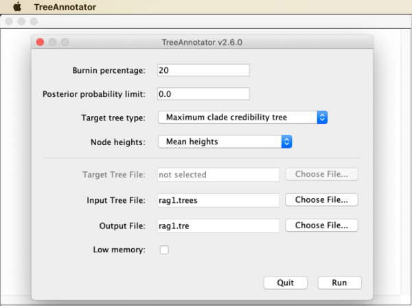
- To generate a more representative tree summarizing the information from the posterior tree distribution, open the program TreeAnnotator which is part of the BEAST 2 package. You should see a window as shown below.

-
Specify a burnin percentage according to the trace plots that we inspected earlier in Tracer (20 in the case of my analysis). Leave the default options for “Posterior probability limit” and “Target tree type” to generate a “Maximum clade credibility tree” (this is the most commonly used type of summary tree for Bayesian analyses; described in Heled and Bouckaert 2013). However, as “Node heights”, choose “Mean heights” rather than the default “Common Ancestor heights”. As input file, select
rag1.treesand specifyrag1.tre(note the different extension) as the output file. When the window looks as shown in the next screenshot, click “Run”.
Visualizing the tree with FigTree
-
When TreeAnnotator has finished (after a few seconds), close the program and open the new file
rag1.trein FigTree. To see the support values for each node, set a tick next to “Node Labels” in the menu on the left, and click on the triangle next to it. Then choose “posterior” from the drop-down menu to the right of “Display”. The posterior node support values represent our confidence that a given node is monophyletic, under the assumption that the employed model is correct. As shown in the next screenshot, most nodes are well-supported.

Help needed?
- To add a time scale to the phylogeny, set a tick next to “Scale Axis” in the menu on the left, but remove the one next to “Scale Bar”. Also click the triangle next to it, remove the tick next to “Show grid” in the newly opened menu field, but set a tick next to “Reverse axis” instead. The result is shown in the next screenshot.

- To also see the confidence intervals for the age estimates, click on the triangle next to “Node Bars” in the menu on the left. Also set a tick in the checkbox for “Node Bars”. Choose the first item from the drop-down menu for “Display”, the “height_95%_HPD” (“HPD” = “highest posterior density”; this is the most common measure of the confidence interval in a Bayesian analysis). You should then see blue bars on each node, these indicate the age range within which the node lies with 95% certainty. The phylogeny should then look as shown below.

SNP filtering
Now that we’ve familiarized ourselves with the most important programs of the BEAST 2 package, we’ll start to prepare the SNP dataset for species-tree inference with the multi-species coalescent model. This dataset of SNP variation for the above-listed 22 individuals of 11 cichlid species is stored in compressed variant-call format (VCF) in file NC_031969.vcf.gz (“NC_031969” is the NCBI accession number for tilapia chromosome 5).
-
Either use
scp [email protected]:workshop_materials/28_species_tree_inference/data/NC_031969.vcf.gz .to copy the file to your own machine or copy it into the directory for this activity on your Amazon instance withcp ~/workshop_materials/28_species_tree_inference/data/NC_031969.vcf.gz .or Guacamole.
As mentioned above, SNAPP is unfortunately very computationally demanding, making the analysis of more than a few thousand SNPs extremely challenging.
Help needed?
bcftools stats NC_031969.vcf.gz (look for “number of records” close to the top of the output) or bcftools view -H NC_031969.vcf.gz | wc -l. A pure UNIX solution would be gunzip -c NC_031969.vcf.gz | grep -v "#" | wc -l. The number of sites should be 430,552.
Help needed?
bcftools stats NC_031969.vcf.gz shows, all records are SNPs; indels have been excluded at an earlier stage.
Help needed?
bcftools stats NC_031969.vcf.gz. Apparently, the VCF file contains 13,174 multiallelic SNP sites.Given that SNAPP can only handle bi-allelic SNPs and only hundreds to thousands of these, we first need to trim down the dataset. Given that we have to exclude some data, we can use the opportunity to select the most useful subset of SNPs for phylogenetic analyses. While filtering for criteria like minor allele frequency could lead to bias in the inference with SNAPP, we can certainly filter for the proportion of missing data or genotype quality. For our first SNAPP analysis, however, we’ll also reduce the number of species to shorten the run time.
-
To reduce the dataset to individuals of the four Neolamprologus species N. marunguensis, N. gracilis, N. pulcher, and N. olivaceous while at the same time excluding multi-allelic sites and sites that are not bi-allelic, use the following command:
bcftools view -s "JWH3,JWH4,JWH1,JWH2,ISA6,ISB3,JWH5,JWH6" -m 2 -M 2 -O z -o NC_031969.s1.f1.vcf.gz NC_031969.vcf.gz -
In the next step, also exclude sites that are monomorphic among the sample (these may have been marked as bi-allelic if all samples differ from the reference), sites that have missing data, and sites with low-confidence genotypes using the following command:
bcftools view -e 'AC==0 || AC==AN || F_MISSING > 0 || QD < 35' -o NC_031969.s1.f2.vcf NC_031969.s1.f1.vcf.gz
(note that with this command, we write an uncompressed VCF output file — after all this filtering, the file size is no longer an issue)
Help needed?
bcftools view -H NC_031969.s1.f2.vcf.gz | wc -l tells us, there are 609 sites left after applying these filters. This number of sites is on the low side but should now be sufficient for our purpose. A good target number of sites for SNAPP analyses is 1,000 - 10,000.-
While we're at it, we'll also prepare another filtered dataset with all 11 species that we'll use later in the second SNAPP analysis. However, to shorten the run time of the analysis, we'll include only one individual per species. Thus, use the following commands:
bcftools view -s "IZA1,JUH9,KHA7,IVE8,JWH1,JWG8,JWH3,JWH5,ISA6,ISA8,KFD2" -m 2 -M 2 -O z -o NC_031969.s2.f1.vcf.gz NC_031969.vcf.gz
bcftools view -e 'AC==0 || AC==AN || F_MISSING > 0 || QD < 35' -o NC_031969.s2.f2.vcf NC_031969.s2.f1.vcf.gz
Help needed?
You should now have two different filtered VCF files prepared for SNAPP analyses: NC_031969.s1.f2.vcf with 609 bi-allelic SNPs for 2 individuals of each of 4 species, and NC_031969.s2.f2.vcf with 702 bi-allelic SNPs for 1 individual of each of 11 species.
Species-tree inference with SNAPP
In this part of the activity, we are going to run a standard SNAPP analysis with the first filtered SNP dataset. As SNAPP is an add-on package to BEAST 2, it also requires input files in XML format; however, the structure of these XML files is quite different from other BEAST 2 XML files. The SNAPP add-on package therefore also includes code that modifies the graphical user interface of BEAUti, so that this interface can be used to easily set up SNAPP XML files. As we will see, however, the model that can be set up through BEAUti has some limitations.
Setting up the SNAPP XML input file with BEAUti
As a very first step, we'll need to make sure that SNAPP add-on package is installed; this can be done through BEAUti's Package Manager.
- Click on "Manage Packages" in BEAUti's "File" menu, and find the SNAPP packaage in the pop-up window with a list of available packages, shown in the next screenshot.

- If, as in the screenshot there is no number next to "SNAPP" in the second column (the one that is titled "Installed" and completely empty in the screenshot), then click on "Install/Upgrade" to install the SNAPP package. After a short moment, you should see a message indicating that the package was installed and that you need to restart BEAUti to see changes to its interface. Click "OK" and restart BEAUti.
- When you now hover with the cursor over "Template" in BEAUti's "File" menu, you should see that a template named "SNAPP" is now available, as shown below.

- Select the SNAPP template. The BEAUti interface should then change, as shown below.

-
There is one more problem to address before setting up the SNAPP XML with BEAUti. As with other BEAST 2 analyses, BEAUti expects input data to be in Nexus format; however, the filtered SNP dataset is in VCF format. We thus need to convert the dataset into Nexus format. One option to do that is by using the Python script
vcf2phylip.py, kindly provided by Edgardo M. Ortiz on his Github repository. Download this script into your activity directory with the following command:
wget https://raw.githubusercontent.com/edgardomortiz/vcf2phylip/master/vcf2phylip.py
(on Mac OS X,curl https://raw.githubusercontent.com/edgardomortiz/vcf2phylip/master/vcf2phylip.py > vcf2phylip.pycould also be used as an alternative towget).
-
Use the
vcf2phylip.pyscript to convert the first filtered dataset to Nexus format. Use the-poption to turn off the default output in Phylip format and the-boption to enable binary Nexus format output, as required by SNAPP:python vcf2phylip.py -i NC_031969.s1.f2.vcf -p -b
-
The
vcf2phylip.pyscript should now have written a file namedNC_031969.s1.f2.min4.bin.nexus. Make sure that this file is present in the current directory. -
Have a quick look at the Nexus file, either using a text editor or the
lesscommand:less -S NC_031969.s1.f2.min4.bin.nexus
You should see that genotypes are now encoded by 0s, 1s, and 2s, which is the format expected by SNAPP.Q What is the frequency distribution of 0s, 1s, and 2s (= how many 0s, 1s, and 2s are in the data matrix)?
Help needed?
One way to count the numbers of 0s, 1s, and 2s are the following commands:
head -n 14 NC_031969.s1.f2.min4.bin.nexus | tail -n 8 | tr -s " " | cut -d " " -f 2 | grep -o 0 | wc -l
head -n 14 NC_031969.s1.f2.min4.bin.nexus | tail -n 8 | tr -s " " | cut -d " " -f 2 | grep -o 1 | wc -l
head -n 14 NC_031969.s1.f2.min4.bin.nexus | tail -n 8 | tr -s " " | cut -d " " -f 2 | grep -o 2 | wc -l
Q Can you tell what each of the three numbers encodes?
Help needed?
Genotypes homozygous for the reference allele are encoded with 0s, heterozygous genotypes are encoded with 1s, and genotypes homozygous for the alternative allele are encoded with 2s. Note, however, that it is irrelevant for SNAPP which is the reference and alternative allele; you could replace all 0s with 2s and vice versa and you should obtain the same result.
- The Nexus file is now ready to be imported into BEAUti. Use "Add Alignment" in BEAUti's "File" menu to do so. The BEAUti window should then look as shown below.

-
By default, BEAUti has tried to assign species IDs to each indiviual, but we know better than BEAUti which individual belongs to which species. Use the table provided above to specify the correct species IDs.
Help needed?
With the correct species IDs, the BEAUti window should look as shown below:

- Move on to the tab titled "Model Parameters". As you'll see the SNAPP model does not appear to have many parameters. In fact, it only contains two parameters (named "u" and "v") for substitution rates, a parameter for the population size named "Coalescent Rate" (in standard SNAPP analyses, this parameter is actually a set of values for the population sizes of each branch), and a parameter for the speciation rate, in addition to the parameters of the species tree (topology and branch lengths). The SNAPP model is thus similarly simplistic as the model that we used for the previous BEAST 2 analysis: It also allows neither extinction nor substitution-rate variation among branches, and it includes only two different substitution types. The difference, however, is that extinction, rate variation, and further substitution types could be added to the model in most BEAST 2 analyses (we just didn't do that because it would have slowed down the analysis), but not in SNAPP analyses. The mathematical framework underlying SNAPP is just so specific that any extension would be difficult to implement and also computationally even more demanding to run.
- Standard SNAPP analyses do not implement a clock model other than the two substitution rates "u" and "v". If we would know, specifically for our dataset, the absolute rate at which 0s turn into 1s and vice versa, we could in principle use these known absolute rates for the two parameters to allow time-calibration of the tree. However, due to ascertainment bias and filtering, there is usually no way to tell the absolute rates for a SNP-only dataset. Thus, we should not even try to estimate a tree with branch lengths according to absolute time, and instead set up the analysis so that branch lengths are in units of substitutions. It is also of little use to allow different values for "u" and "v"; thus, we fix both rates at 1. To do so, remove the tick on the right of "Mutation Rate U", next to "Sample". This will mean that throughout the MCMC inference, the two parameters will remain at their initial values, which are entered in the fields next to rates as "1.0" in both cases.
- Also specify 1.0 as the initial value for the "Coalescent Rate" parameter, but do not remove the tick next to "Sample" to the right of this parameter.
- Finally, make sure to remove the tick next to "Include non-polymorphic sites", given that all sites in our dataset are variable. The BEAUti window should then look as shown in the next screenshot.

-
Now move on to the "Prior" tab. Here, you can specify prior distributions for those parameters of the model that we did not fix, the speciation rate lambda and the population size parameter. The way this population size parameter is used is a bit confusing in SNAPP. In the "Model Parameters" tab, we set an initial value of 1.0 for the "Coalescence Rate" but the prior distribution that we can now specify is for the population mutation rate "Theta" (Θ = 4 Ne μ; four times the effective population size Ne times the per-generation mutation rate μ). The two items, however, are just two aspects of the same parameter, as SNAPP calculates Θ as 2 divided by the coalescence rate (see source code). Another confusing inconsistency is that both the initial value and the prior distribution for lambda are specified in this tab whereas we specified the initial values for other parameters already in the previous tab. We'll keep the defaults for both the initial value and the prior distribution for lambda. However, the default values for the population size parameter are rather arbitrary and should be changed. With SNP data from multiple species, it is extremely difficult to develop a prior expectation for the population size parameter, as Theta depends on the mutation rate, which is subject to ascertainment bias in such datasets. Because invariant sites are not included in a SNP dataset, SNP datasets necessarily appear more variable than the whole-genome dataset from which the SNPs were derived, and thus the mutation rate of the SNP data appears exaggerated. While SNAPP implements a correction for ascertainment bias, simulations that we performed in Stange et al. (2018) showed that the true genome-wide Theta can not be recovered even with this correction (however, estimates of branch lengths and topology are nevertheless accurate).
To avoid unintended effects of the prior, I therefore recommend to use a wide and uninformative prior distribution for the population size parameter. The type of this distribution can be set from the drop-down menu next to "Rateprior" where initially a gamma distribution is selected. The entries for "Alpha" and "Beta" above this drop-down menu define the shape of this gamma distribution. The "Kappa" value, however, is only used when the "CIR" distribution is selected from the drop-down menu; otherwise, the value specified for "Kappa" is ignored by SNAPP. Instead of the gamma distribution, select "uniform" from the drop-down menu to apply a uniform prior. Unlike in other types of BEAST 2 analyses, the boundaries of this uniform distribution can not be adjusted in BEAUti; instead they are hard-coded in the source code of SNAPP. When the uniform distribution is selected, all the values entered for "Alpha", "Beta", and "Kappa" are ignored. The BEAUti window should then look as shown below.

- Continue to the "MCMC" tab. With SNAPP, a much shorter chain length is usually required than for other types of BEAST 2 analyses, given that few parameters need to be estimated and that the computation is much slower. Set a chain length of "50000" and specify "50" next to "Store Every" to reduce the frequency at which states are stored (in a backup file with the ".state" ending — this file can be used to resume an interrupted analysis). Also click on each of the three black triangles on the left and specify "50" next to each "Log Every" as the frequencies at which output is written to the screen and to the ".log" and ".trees" files. Instead of the defaul names for the ".log" and ".trees" output files, specify "s1.log" and "s1.trees". The BEAUti window should then look as shown in the next screenshot.

-
Finally, save the XML file for SNAPP by clicking "Save" in BEAUti's "File" menu and name the file
s1.xml.
If anything went wrong during the generation of the XML file for SNAPP, you can find a precomputed version of file s1.xml in directory ~/workshop_materials/28_species_tree_inference/res on the Amazon instance and continue the next steps of the activity with it.
Running SNAPP
Running SNAPP works exactly the same way as running BEAST 2.
-
If you run BEAST 2 on your own Mac OS X or Linux machine (if not, read the next point), open the program again (first close it if it was still open), click "Choose File...", and select file
s1.xmlas the input file. If the computer on which you run this analysis has multiple CPUs and these are available, you could also specify that more than one thread should be used; this will speed up the analysis. To do that, click on the drop-down menu next to "Thread pool size:" and select a number according to the available CPUs. The BEAST 2 window should then appear as in the next screen shot. Click "Run" to start the MCMC inference.

-
If you run BEAST 2 on your own Linux machine or on the Amazon instance through Guacamole, use again a terminal (such as the MATE Terminal on the Amazon instance) to navigate to the XML file with the
cdcommand, and launch BEAST 2 withbeast -threads 4 s1.xml(use four threads on the Amazon instance or another number of threads on your own machine according to its number of CPUs). - The BEAUti 2 screen should then show continuously updating numbers as in the earlier BEAST 2 analysis, similar to the output shown in the following screenshot.

Help needed?
- The sequentially increasing states of the MCMC (only every 50th state is shown).
- The logarithm of the posterior probability (= the likelihood of the result multiplied by the prior probability) of the result given the parameter values at a certain state.
- An approximation of the ESS value for the posterior up to a given state.
- The logarithm of the likelihood of the result given the parameter values at a certain state.
- The logarithm of the prior probability of the parameters at the state.
- A prediction for the run time per million states based on the run time required so far.
Help needed?
If the SNAPP analysis looks like it is going to run longer than you are willing to wait, you could in the meantime take a coffee break or continue with section Divergence-time estimation with SNAPP before coming back to the next part, Postprocessing SNAPP results. Instead of running the MCMC on your own machine, you could also use precomputed versions of files s1.log and s1.trees, which you can find in directory ~/workshop_materials/28_species_tree_inference/res on the Amazon instance. Note, however, that these files were generated with a longer chain length of 1 million states.
Postprocessing SNAPP results
-
Open the log file written by SNAPP,
s1.login Tracer and click on the "Trace" tab in the top right of the window to see the MCMC trace for the posterior probability. The window should then look as shown in the screenshot below.

- Adjust the burn-in if necessary. In the case of my analysis shown above, the burn-in could be set to 10,000, which is roughly the state at which the plateau in the posterior trace was reached.
Help needed?


If you'ld like to explore these results in more detail, you could use the log file of the longer analysis,
s2.log, which you can find in directory ~/workshop_materials/28_species_tree_inference/res on the Amazon instance, and open it in Tracer.- Also have a look at the trace plots for some of the Theta parameters. Each Theta parameter corresponds to the population size estimate for one of the branches of the tree. You'll probably see traces that look like the one shown in the next screenshot.

Trace plots like the one shown above indicate that some of the Theta parameters are difficult to estimate, presumably because the data contains little information about them. It is likely that those traces with the lowest ESS values are for internal branches of the tree, where population sizes are generally more difficult to estimate than for terminal branches. This problem could probably be fixed by adding data from more individuals per species to the dataset, but it would in contrast be probably more severe if we would have more species included and thus more internal branches relative to terminal branches.
-
Again use TreeAnnotator to generate a summary tree for the first SNAPP analysis, with the same settings as before for the BEAST 2 analysis. Thus, adjust the burn-in percentage according to the trace plot for the posterior probability, select "Mean heights" from the drop-down menu for "Node heights", use file
s1.treesas the input file, and name the output files1.tre. -
Open the file with the summary tree,
s1.tre, in FigTree.

Help needed?
- Display node support in FigTree by setting a tick next to "Node Labels", clicking on the triangle to the left of it, and choosing "posterior" from the drop-down menu next to "Display".
- Also display the Theta estimates on branches by setting a tick next to "Branch Labels", clicking on the triangle to the left of it, and choosing "theta" from the drop-down menu next to "Display". A bit below this drop-down menu, replace "4" with "10" in the field next to "Sig. Digits" to display more decimal positions for th Theta estimates. Compare the node support and the Theta estimates in your species tree with those from my analysis, shown below.

Help needed?
As noted above, the Theta values inferred by SNAPP are difficult to interpret in absolute terms due to ascertainment bias. In the next part of this activity, we'll see how SNAPP can be tuned to allow estimates of divergence times and effective population sizes on an absolute scale.
Divergence-time estimation with SNAPP
In this part of the activity, we are going to specify a customized model for SNAPP to estimate the species tree of the second SNP dataset, composed of data from 11 cichlid species. This model was explored in detail in our paper on catfish divergences related to the closure of the Panamanian Isthmus (Stange et al. 2018). It differs from SNAPP's standard model primarily by including a (strict) clock model and by linking the Theta estimates of all branches. The latter choice was made mainly to speed up the analysis, as particularly with datasets of larger numbers of species, the Theta values make up most of the complexity of the model. By linking all Theta values we also avoid the issue of low information content for the estimation Theta values of internal branches that was mentioned above. Of course, a consequence of linking all Theta values is that differences in the population sizes among species can no longer be accounted for, but this may be seen as a reasonable compromise to make in exchange for the much faster run times that can be achieved that way.
Setting up the XML input file with snapp_prep.rb
This customized model for SNAPP can unfortunately not be specified through the graphical user interface of BEAUti. Instead, XML files implementing this model can be written with the Ruby script snapp_prep.rb that we developed for our work for Stange et al. (2018).
-
Download the content of the Github repository for the
snapp_prep.rbscript, for example using the following command:
git clone https://github.com/mmatschiner/snapp_prep.git -
Have a quick look at the content of the downloaded directory, for example using
ls -l snapp_prep. You should see that it includes the scriptsnapp_prep.rb, another script namedadd_theta_to_log.rb, a number of example files, and a (short) README file. -
Move the content of the downloaded directory into the current directory, using the following command:
mv -f snapp_prep/* .; rm -rf snapp_prep -
Have a look at the content of the example files
example.spc.txtandexample.con.txt, either using a text editor or thelesscommand. You'll see that the first of the two files contains a table assigning individual IDs to species IDs, and the second includes time constraints and some explanation about these. To understand the way in which these time constraints can be used, you could read through these explanations, but note that we are only going to use a simple normal distribution as a time constraint in this activity, which will be described below. -
To test the Ruby script and see its help text, run the following command:
ruby snapp_prep.rb -h
From the displayed options you should see that input can either be specified in Phylip format with "-p" (this format is similar to the Nexus format used above) or in VCF format with "-v". In addition, the table assigning individual IDs to species IDs must be specified with option "-t" and a file with time constraints must be given with option "-c". Other options that will be important for us are "-l" to set the length of the MCMC, "-x" to specify the name of the resulting XML file, and "-o" to specify how the ".log" and ".trees" output files should be named by SNAPP. Options that could be useful in other cases but that we will not use here are "-m" to limit the number of SNPs and "-r" and "-i" to include only transversions or only transitions, respectively. Splitting the dataset into transitions and transversions could help to compensate at least to some degree for the simplistic substitution model of SNAPP, which assumes that all types of substitutions occur with the same rate. -
Open a text editor and prepare an input table for the script that is equivalent to the table in file
example.spc.txt, linking individual IDs and species IDs. Write the following content (with either a space or a tab symbol between the columns), which is based on the table provided above but limited to the one individual per species that we included in the second filtered SNP dataset:species specimen astbur IZA1 neobri JUH9 neochi KHA7 neocra IVE8 neogra JWH1 neohel JWG8 neomar JWH3 neooli JWH5 neopul ISA6 neosav ISA8 neowal KFD2 Save this file with the name
s2.spc.txt -
Next, also write a file equivalent to the example file with time constraints,
example.con.txt. To specify a normal prior distribution on the age of the root of the species tree, write the following text to this file: "normal(0,7,0.1) crown astbur,neobri,neochi,neocra,neogra,neohel,neomar,neooli,neopul,neosav,neowal" (with a space or a tab before and after "crown"). The normal prior distribution then has an offset of 0, a mean of 7, and a standard deviation of 0.1; in millions of years, these ages roughly correspond to recent findings for the age of these species. By listing the IDs of all species in the dataset, we define that the constraint is placed on the (crown) age of the group comprising all these species and thus on the root of the species tree. -
On a second line of the same file, write the following text: "monophyletic NA neobri,neochi,neocra,neogra,neohel,neomar,neooli,neopul,neosav,neowal". With this text, we do not specify another time constraint, but a constraint on the topology which enforces the monophyly of the listed species. By here listing all species IDs except "astbur", we define a clade comprising all species except Astatotilapia burtoni and we thus make Astatotilapia burtoni the outgroup to all others, which is strongly supported by previous studies. Save the file with the name
s2.con.txt. -
With the files
s2.spc.txtands2.con.txtprepared, we can now use these as input tosnapp_prep.rb. To also specify an MCMC length of 100,000, "s2.xml" as the name of the XML file, and "s2" as part of the ".log" and ".trees" files that will be written by SNAPP, use the following command:
ruby snapp_prep.rb -v NC_031969.s2.f2.vcf -t s2.spc.txt -c s2.con.txt -l 100000 -x s2.xml -o s2
This should finish within a second. The script is going to issue a warning that no starting tree has been specified which could sometimes make it difficult for SNAPP to start the inference. It is difficult to predict when this is the case, so let's first try without a starting tree and see if SNAPP requires one.
Running SNAPP
-
If you run this activity on your own Mac OS X or Windows machine (if not, skip this point), open BEAST 2 once again (if it is still open, close and reopen BEAST 2), select the XML file written by
snapp_prep.rb,s2.xml, increase the number of threads if possible, and then click "Run" to start the SNAPP analysis. -
If you run the activity on your own Linux machine or on the Amazon instance through Guacamole, again navigate to the directory in which
s2.xmlis placed withcdand launch BEAST 2 with e.g.beast -threads 4 s2.xml.
Help needed?
s2.starting.tre: "(astbur:7,(neobri:3,neochi:3,neocra:3,neogra:3,neohel:3,neomar:3,neooli:3,neopul:3,neosav:3,neowal:3):4);". If you're curious to see how the starting tree looks like, you could open it in FigTree. Use snapp_prep.rb once again to write the SNAPP XML file, this time providing the starting tree file with the option "-s":ruby snapp_prep.rb -v NC_031969.s2.f2.vcf -t s2.spc.txt -c s2.con.txt -l 100000 -x s2.xml -o s2 -s s2.starting.treThen, try again to open and run the XML file with BEAST 2. This time, the SNAPP analysis should start to run.
- Follow the screen output for a while until the estimated time required per million samples is reported in the last column of the output. When this time is reported for the first time, make a rough calculation how long the analysis will take.
Help needed?
-
If you don't have that much time to spare, feel free to cancel the analysis and continue the rest of the activity with precomputed output files of this analysis. These output files (
s2.logands2.trees) can be found in directory~/workshop_materials/28_species_tree_inference/reson the Amazon instance, but note that these output files were generated with a longer chain length of 400,000 states.
Postprocessing SNAPP results
-
Once BEAST 2 has finished the MCMC analysis (or as soon as you got too tired of waiting or when you decided to use the precomputed output files instead of your own), open file
s2.login Tracer. If you then click on the "Trace" tab at the top right of the window and adjust the number of burn-in states, you should see something similar to the screenshot below.

In contrast to the previous SNAPP analysis, the log file now includes a parameter named "clockRate", which obviously estimates the rate of the strict molecular clock. However, like for the Theta parameter, the estimate for the clock rate is also commonly affected by ascertainment bias (Stange et al. 2018) and therefore can't usually be considered reliable. Besides, the ESS value for the clock rate parameter is still low, and its trace does not appear to be stationary yet, as shown in the next screenshot.

As you may also notice, the estimates for Theta are not included in the log file, unlike in the first SNAPP analysis. The reason for this is that the snapp_prep.rb script wrote the SNAPP XML so that Theta values are excluded from its log output, because SNAPP would otherwise write identical Theta values for each branch of the tree, which could fill the log file with a lot of redundant information. However, the estimates for Theta are anyway still included in the second output file written by SNAPP, the ".trees" file s2.trees.
-
The script
add_theta_to_log.rb, which was also included in the Github repository for thesnapp_prep.rbscript, can be used to transfer the Theta estimates from files2.treesto a new version of the log files2.log. Before you do so, first have a look a the help text of this script:
ruby add_theta_to_log.rb -h
You'll see that the script expects as input the ".log" and ".trees" files from a SNAPP analysis, to be specified with options "-l" and "-t", respectively. In addition, an estimate of the generation time in years, specified with "-g" is required to calculate an absolute estimate of the population size from the estimates of Theta and the clock rate. And finally, an output file needs to be specified with option "-o", this output file will be in the same format as the input log file, just with additional information. -
Run the script
add_theta_to_log.rbwith the following command to generate a new log file including estimates for Theta and the population size:
ruby add_theta_to_log.rb -l s2.log -t s2.trees -g 3 -o s2_with_theta.log -
Open the newly written log file
s2_with_theta.login Tracer, and once again click on the "Trace" tab in the top right and adjust the number of states considered as burn-in. The Tracer window should then show something similar to the next screenshot.

- As you can see, the list of parameters in the bottom left of the Tracer window now includes estimates for Theta and the population size. Select both "clockRate" and "theta" from the list of parameters and click the tab for "Joint-Marginal" at the top right. You should then see that both of these parameters are highly correlated, as shown in the next screenshot.

Based on the simulations that we performed for Stange et al. (2018), SNAPP's estimates for the population size in general appear to be accurate (at least under the assumption that the multi-species coalescent approximates evolution well), in contrast to those for Theta and the clock rate, which are affected by ascertainment bias. Thus, if we ignore the very low ESS value for the population size estimate (which tells us that we should extend the MCMC chain), we can interpret these results as evidence for a population size of cichlids around 30,000. A second parameter of possible interest is the speciation rate lambda, estimated around 0.6, which means that per million year, the probability that a species in the tree speciates is around 0.6 (note, however, that this estimate is only reliable under the assumption that the dataset includes all species of a taxonomic group).
-
Finally, use TreeAnnotator again to generate a summary tree for this second SNAPP analysis. As before, adjust the burn-in percentage according to the trace plot for the posterior in Tracer, select "Mean heights" from the drop-down menu for "Node heights", use file
s2.treesas the input file, ands2.treas the name of the output file. -
Open the summary tree file,
s2.tre, in FigTree. As with the first summary tree generated by BEAST 2, add a reverse time axis and display node ages as node labels. To also display the uncertainty in node ages, set a tick next to "Node Bars", click on the triangle to the left of the tick box, and choose "height_95%_HPD" from the drop-down menu next to "Display". The FigTree window should then appear as shown in the screenshot below.

- Also inspect the node support by clicking on the triangle next to "Node Labels" once again, and selecting "posterior" from the drop-down menu next to "Display".
Help needed?
Further information
This activity is in part based on more extended tutorials available on https://github.com/mmatschiner/tutorials, in particular the tutorials Bayesian Phylogenetic Inference and Divergence-Time Estimation with SNP Data. Thus, if you'ld like to learn more about BEAST 2 and SNAPP analyses, you could also follow those tutorials. The BEAST 2 website also provides a wide range of tutorials and manuals. In addition, you can find many further tutorials on the Taming the BEAST website, where you will also find information about the excellent Taming-the-BEAST workshops. Finally, if you have further questions regarding BEAST2, you could have a look if somebody else already asked those questions on the very active user forum, or you could ask these questions there yourself.