
Inferring population recombination rate from population data
Marion Talbi and Milan Malinsky, 08 January 2025
Background and Objectives
Every generation, recombination shuffles regions of the genome with different patterns of genetic diversity together, generating new haplotypes that natural selection can act on. Thus, both the rate and the distribution of recombination have an impact on the strength of selection, and can influence the speed and dynamics of adaptation and speciation. It is therefore a worthy parameter to obtain in population genomic studies.
To infer recombination, different methods are available (see This review from Peñalba and Wolf (2020) for more background).
With the increasing availability of population genomic data, LD-based methods have demonstrated a great ability to infer the fine-scale recombination rate. These methods use the patterns of distribution and association of polymorphism present in population genetic data within the theoretical framework of the coalescent to infer the population recombination rate, ρ. We refer to the population recombination rate because the patterns of LD that we observe are a result of the product of the per-gene-per-generation recombination rate r, and the effective population size Ne.
In this activity, we will use the software
Table of contents
- Inference of the demographic history for each population
- Inference of fine-scale recombination rates
- Visualisation with RStudio
Github:
Material
All material files are available here ~/workshop_materials/21_recombination_estimation.
Workflow
I. Inference of the demographic history
As said earlier, ρ is encapsulating both r and Ne, thus, variation in Ne will impact our estimates of ρ.
We thus need first to infer past changes in demography.
In this activity, we will use smc++ (other methods are available, e.g. see MSMC, or fsc2 – activity to come soon).
smc++ used the SCM classical algorithm (from PSMC) with the site frequency spectrum of all other individuals as the observed state. (But read Terhost et al., 2017. Robust and scalable inference of population history from hundreds of unphased whole genomes for more background)
Inferring change in demography with smc++ is a straightforward three steps method, but first, use the following command to access the command on your instance:
source /home/wpsg/smcpp/bin/activate
And this one to move to the good directory:
cd ./smcpp/
Once you did this, you can continue with the next steps.
- Convert VCF to smc++ format:
- Fit a model of population demography changes to the data:
- Plot data and output a csv file:
First, we want to prepare the input file using the following commands:
Show me the commands
vcf=../input_files/Astac_LS420024.2.vcf.gzzcat ${vcf} | sed 's/\t\.:/\t\.\/\.:/g' | bgzip > Astac_LS420024.2.smc.vcf.gzThis sed command is changing how missing data are encoded in our VCF.
bcftools index Astac_LS420024.2.smc.vcf.gz
This command is creating an index for our VCF.
vcf_smc=./Astac_LS420024.2.smc.vcf.gz
This is the input VCF that you will need to run smc++.
Then, you can try to run the following commands: (all the commands you’ll need are in the
vcf_smc=./Astac_LS420024.2.smc.vcf.gz #We save the name of a VCF into a variable
chr=LS420024.2 #Same for the chr number
##Benthic pop
smc++ vcf2smc ${vcf_smc} ${chr}_BEN.smc.gz ${chr} BEN:D29A01,D29A02,D29A03,D29A04,D29A05,D29A08,D29A09,D29B01,D29B02,D29B03,D29B05,D29B06,D29B07,D29B08,D29B10,D29C01,D29C04,D29C05,D29C07,D29C08,D29C09,D29C10,D29D01,D29D02,D29D03,D29D04,D29D06,D29D07,D29D08,D29D09,D29D10,D29E01,D29E02,D29E03,D29E04,D29E05,D29E06,D29E07,D29E08,D29F01,D29F02,D29F03,D29F04,D29F05,D29F06,D29F07,D29E09,D29E10,D29F08,D29F09,D29F10,D29G02,D29G03,D29G04,D29G05,D29G06,D29G07,D29G08,D29G09,D29G10,D29H01,D29H03,D29H04,G03I01,G08A03,G08A05,G08B05,G08B07,G08C03,G08D01
##Littoral pop
smc++ vcf2smc ${vcf_smc} ${chr}_LIT.smc.gz ${chr} LIT:D31B06,D31B07,D31B08,D31B09,D31B10,D31E04,D31E05,D31E06,D31E09,D31E10,D31F01,D31F02,D31F03,D31F04,D31F05,D31F06,D31F07,D31F08,D31F09,D31F10,D31G01,D31G02,D31G03,D31G04,D31G05,D31G06,D31G07,D31G08,D31G10,D31H01,D31H02,D31H03,D31H04,D31H05,D31H06,D31H07,D31H09,D31H10,D31I06,D31I07,D31I08,D31I09,D31J01,D31J02,D31J03,G01B03,G02D08,G03F07,G04C05,G04D04,G04H05,G05D06,G05H07,G05I01,G05I04,G05J08,G08I05,G08J04,G09A05,G09B09,G09C02,G10G06,G10G07,G10G10,G10H03,G10H04,G10H05,G10H06,G11A07
This is creating the smc input file for both populations.
the mask command
--mask is optional, but can be used to focus only on non-coding region of the genome for example. In real life – you might want to exclude some regions of the genome from your analysis. (e.g. low quality regions or regions undergoing selection). In the folder, you will find the file Astac_allMasksandCodingregions.bed.gz. This is a bed file including regions with low mappability, missing individuals, regions consider as low quality by GATK, and regions with extrem depths (both too high or too low). This mask also includes coding regions of the genome, because these regions might be under positive selection).
--mask command, and compare the inferences obtained with and without the mask.
Show me the command
mu=3.5e-9
smc++ estimate --base LS420024.2_estimate_BEN -o ./ ${mu} LS420024.2_BEN.smc.gz

smc++ estimate --base LS420024.2_estimate_LIT -o ./ ${mu} LS420024.2_LIT.smc.gz
This step is a bit long to run, you can try of course, but the output file is already in the folder
Show me the command
cd ./output_files ) and run the following command:chr=LS420024.2
smc++ plot --csv ${chr}_BENLIT_smcpp.pdf ${chr}_estimate_BEN.final.json ${chr}_estimate_LIT.final.jsonShow me the answer!
We now should have a csv file and a pdf file with population sizes through time.
The csv file displays the name of the population, the time in generation, and the corresponding effective population size for this time interval.
In the folder, you will find two other output files from smc++:
- One run on the chromosome 4 (i.e. LS420022.2):
./smcpp/output_files/LS420022.2_BENLIT_smcpp.csv - One run on all the chromosomes:
./smcpp/output_files/All_chromosome/All_chromosome_BENLIT_smcpp.csv
Show me the answer!

II. Inference of fine-scale recombination rates
For this part, we will need to use
To access it on your instance, you will need to activate the following conda environment:
conda activate pyrho
And to move in the good directory:
cd ~/workshop_materials/21_recombination_estimation/pyrho/
- Lookup tables construction
- Fine-scale recombination rates inference
- The block-penalty: Used to determine the smoothness of a map.
- The window-size w: Determines how far appart can be the SNPs before being ignored.
The software LDpop is used to built the lookup table – i.e. the table with all two-locus likelihoods to observe a grid of values of ρ given one mutation rate. This software is, compare to older ones (see LDhelmet), implementing changes in demography in the likelihoods estimation.
Here is the code to use. As we run earlier smc++, we can now add the changes of demography to obtain more accurate lookup tables.
pyrho make_table --samplesize [nhaplotypes] --approx --moran_pop_size [Nmoran] --mu [mutation_rate] --outfile [out.name] --popsizes [pop_sizes] --epochtimes [epochtimes]
Show me the answer!
You can open this file with this command:
less ~/workshop_materials/21_recombination_estimation/pyrho/scripts/script_pyrho_table.sh
Or, if you know how to exit
vi ~/workshop_materials/21_recombination_estimation/pyrho/scripts/script_pyrho_table.sh
Then, the final commands with all arguments are:
pyrho make_table --samplesize 138 --approx --moran_pop_size 200 --mu 3.5e-9 --outfile ./output_files/69_pyrho_lookuptable_littoral --popsizes 75996,25195,12907,5699,6792,21764,84371,177574,103772 --epochtimes 1943,2484,2880,4134,7441,18379,54395,112126
and
pyrho make_table --samplesize 140 --approx --moran_pop_size 200 --mu 3.5e-9 --outfile ./output_files/70_pyrho_lookuptable_benthic --popsizes 72630,12907,5699,6792,21764,84371,177574,103772 --epochtimes 2006,2880,4134,7441,18379,54395,112126
This step is pretty long to run. You will find the output files in
Use of composite-likelihood and fused-lasso to infer the population recombination rates.
There are two important parameters here:
You could for example use simulation to find the most suitable values for these parameters, or you could also use the --hyperparam command of
The command to run
pyrho optimize --vcffile ${vcf} --windowsize ${windowsize} --blockpenalty ${bp} --tablefile ${lookuptable} --ploidy 2 --outfile ${name_output}
Show me the answer!
You can open this file with this command:
less ~/workshop_materials/21_recombination_estimation/pyrho/scripts/script_pyrho_optimize.sh
Or, if you know how to exit
vi ~/workshop_materials/21_recombination_estimation/pyrho/scripts/script_pyrho_optimize.sh
The final commands with all arguments are:
pyrho optimize --vcffile ../input_files/LS420024.2_benthic.vcf.gz --windowsize 50 --blockpenalty 15 --tablefile ./output_files/70_pyrho_lookuptable_benthic --ploidy 2 --outfile ./output_files/LS420024.2_benthic_bp15_pyrho.optimize
and
pyrho optimize --vcffile ../input_files/LS420024.2_littoral.vcf.gz --windowsize 50 --blockpenalty 15 --tablefile ./output_files/69_pyrho_lookuptable_littoral --ploidy 2 --outfile ./output_files/LS420024.2_benthic_bp15_pyrho.optimize
The output file is a three column file. The first column is the start of an interval, the 2nd is the end of the same interval, and the third column is
Extra question
III. Map Visualisation using R Studio
The Rcode for this activity is available here. You could then connect to R-studio, and copy paste this code.
There are different units used to refer to recombination rate. For example,
Another common units used to represent recombination rates is the centiMorgan. One centiMorgan is the genetic distance corresponding to 1% chance of observing one event of recombination.
Show me the answer!
 So here, th recombination rate in cM is equal to
 2.689911e-09 / 0.01 =2.689911e-07.
Show me the answer!
One cM is still equal to 1% chance of observing an event of recombination. Thus 
If we want to convert the output of
You can do so with the following R command: (you will need to adapt the name of the dataset and the name of the variable)
maps$"cM/Mb"<-(maps$rate_r/0.01)*10^6From this frequency of recombination event, we can now obtain the cumulative genetic distance in centiMorgans. It will give information about the total length of the genetic map.
Look at this example:
| Chromosome | Position(bp) | Rate(cM/bp) | Map(cM) |
| chr1 | 2539 | 0.455158616243 | 0.00457837 |
| chr1 | 5806 | 0.375735428466 | ? |
Show me the answer!
You will have:

To find the missing value in the table, you can use this code:
(5806-2539)*(0.455158616243/10^6) + 0.00457837
Now that we have our output in two different units and that we are able to obtain the recombination map in cM, it would be interesting to have a first look at our recombination landscapes.
To do so, we can use
Show me the answer!

We now have our two recombination landscapes. You can see variation along the chromosome, with some regions having more chances to observe an event of recombination (i.e. an higher recombination rate)
Once you managed to do it, you can compare with the maps built with a different value of block penalty.
Show me the answer!

From this plot, we see that the two plots differ with the number and size of ‘spike’. It makes perfect sense, because the block-penalty adds a penalty to big jump along the recombination map.
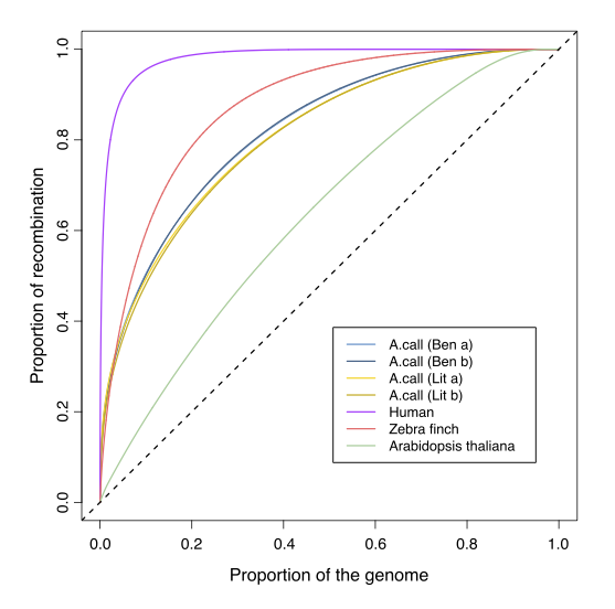
As you might have noticed, the landscape of recombination is not homogeneous along the genome, and when comparing different population/species, we might want to have an idea on how different the landscapes are. The cumulative curve representation is useful to do so:
Show me the answer!
Show me the answer!
