Sequencing is RAD…

It’s interesting to think about “Why do organisms look the way they do?” This question has fascinated scientists all the way back to Aristotle, the whole idea of a unity of type and conditions of existence. Model organisms have been of great importance in research such as understanding cancer using model organisms; specifically studying the development of brain cancer using somatic evolutionary genomics. Essentially, what they did was use laser capture microdissection to isolate cancer cells, did a transcriptomic analysis of different cells and look for genomic rearrangments (which were found). Remember Evan’s talk…inversions and genomic rearrangement impacts in different studies that he talked about. Inversion can have a profound affect.

So whether model or nonmodel organisms we have a series of questions that we want to answer:

• Where does diversity lie in the genome?
• How do organisms adapt to novel environments?
• How is genetic diversity partitioned in individuals, populations and species?
• What genomic regions are important for phenotypic variation that adapts an organism to a novel environment?
• How does the ecology of organisms structure genomic architectures?
• Where does the basis for evolutionary novelty reside in genomes?

We use RAD-seq to get at the questions of the genomic basis behind phenotypic variation in ‘the wild’; we look at Funcitonal Evolutionary Genomics.

There are four fundamental processes in evolution:

1. Mutation
2. Migration
3. Genetic Drift
4. Natural Selection

The first two fall under the origins of genetic variation, the second two under sorting for genetic information.  Genetic drift is thought of here as the NULL model and while it is really an oversimplification of the neutral process it is a good start.

In population genomics we are doing a simultaneous typing of neutral and adaptive loci. Anothewards, we have a genome-wide background of neutrality and that provides more precises estimates of demographic processes and phylogeography. And ‘sticking out’ from this background would be adaptive loci to indicate selective sweeps and local adaptation. So this begs several questions:

• What are the expectations of diversity of genomes in populations?
• How can we group these together so we can look at sequence based variation
• What is the expected pattern of topology given neutral theory and what would you expect when relating it to statistics such as Fst. Do they confirm each other?

How do we genomically enable research studies of nonmodel organisms?  

• We need genetic markers and maps, we need physical maps with at least one reference genome (in the future perhaps we’ll need to use suites of reference genomes). We need transcriptomes to annotate genomes, and we need to understand differences in gene expression levels.

Why not just sequence the entire genome?

• It’s still prohibitively expensive and a lot of times full sequence isnt’ necessary.
• It takes a lot of time.
• Genetic maps can be quite useful and can be used to facilitate genome assembly down the line.

So an alternative approach would be reduced representation NGS genotyping (using reduced representation libraries -RRL). In this we focus sequencing on homologous regions across the genome followed by simultaneous identification and typing of SNPs. The cost is a fraction of what it would cost to sequence a full genome and you can assay 1000’s of genomes in just a few weeks. Lastly, Why not, as stated above complete genomic sequence may not be necessary. Once caveat to be aware of that we’ll touch on more later is that this type of sequencing is not appropriate for phylogenetic analysis on organisms that are more than a few % diverged.

• RRL libraries: all rely on restriction enzyme digestions. RAD-seq specifically uses a shearing step to efficiently capture restriction sites. It incorporates barcodes and/or adaptors for multiplexing, aligns against reference or de novo. There are statistical issues such as sampling variation of sequence as well as  biological and sequencing error and this makes analysis difficult.

RAD-seq: This is a reduced representation next generation sequencing genotyping technique using restriction enzymes where you sequence homologous tags spread throughout the genome.

• You can call SNPs simultaneously
• It’s cheaper
• Better than a SNP chip because a SNP chip may not be applicable to any other organism other than the one you designed it for.
• You can do this on 1000’s of genomes in a matter of weeks
• Reasons not to? If you are trying to analyze a genome that has shorter LD blocks. LD is linkage disequilibrium where you have linked loci. When you are at linkage equilibrium in your genome then essentially there is no linkage in the genomes, everything is random everywhere, shuffling ad hoc. In linkage disequilibrium you have blocks of loci that ‘carry’ each other forward evolutionarily and are conserved or selected for together.

The difference between RAD and other techniques you might have heard of such as CRoPs, MSG or GBS  is that RAD has a shearing step in the protocol to improve mapping and coverage/distribution of your fragments. You use barcoding like the other methods and you can take the output and map it to a reference or assemble the ‘stacks’ de novo.

The flow of RAD-tags is as follows…

1. You have sites within a genome that corresponds to sites that can be cut using a restriction enzyme.
2. Once cut you can ligate the amplification primer, sequencing primer and barcode to the sticky overhang left from the cutting.
3. You can finish the other ‘blunt’ end with an adapter, amplification and sequencing primer to allow for amplification prior to NGS.
4. You then follow the normal protocols for next generation sequencing and get well…a f*!k ton of data to say the least… see figure below…

 

Considerations:

1. Make sure your barcodes are sufficiently different from one another because later on you will be specifying parameters and ‘allowing’ for mismatches. So if you have two barcodes different by one or two nucleotides and you ‘allow’ later on for 1-2 mismatches you’ve effectively made your two distinct barcodes one and same in the eyes of the computer and you will not be able to tell those two samples apart from each other and as Julian stated once…“I’ve done it, it’s a mess”.
2. Through experiementation the Cresko lab has determined that random shearing improves the distribution of coverage across your genome for your sites versus other methods that don’t use a shearing step.
3. Number of sites versus depth versus number of samples. You have to think about the trade offs. You really ought to have 20-50x coverage ideally. Well if you have a million reads, 100x depth, 1000 samples you’ve only got an average coverage/sample of 10x…not ideal. So take this into consideration.
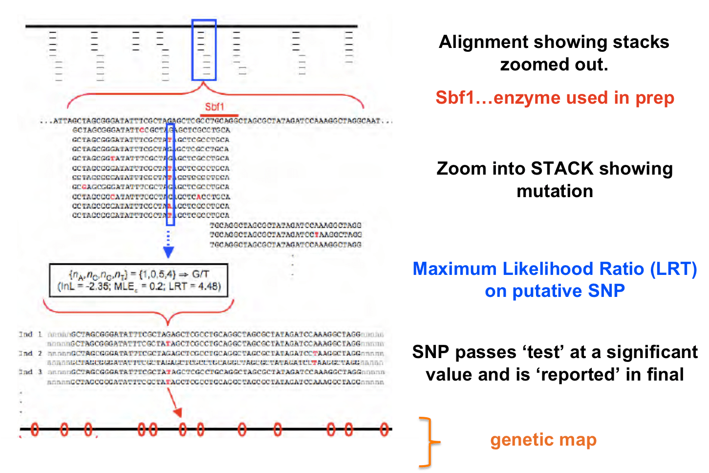
4. Distinguishing true SNPs from sequencing error: RADs uses a maximum likelihood method to determine if SNPs are significant to be ‘called’. But keep the above in mind too…if you’re coverage is still low, your statistical test will no yield significant results for SNPs even though they might be truly there. So keep coverage in mind.
5. The number of barcodes you should use? Well barcodes are typically 5-8 nts long and need to be sufficiently different to be able to sort. So consider that.
6. Don’t ever forget library quality!! If your sequences suck, your downstream processing and analysis will too!
7. You really ought to use qPCR to normalize libraries
8. You need depth across sites and be able to identify what’s error versus what’s a heterzygous SNP and you really should model your base calls.
9. STACKS uses an ML model but Bayesian models can also be used and can be biased depending on the priors you use.
10. There is bias in RADseq and bias is ok as long as you know its there and you know how to account for it.
11. Using RAD seq for phylogeny will be difficult…as you get more divergence the more and more rad sites that will be different. so the number of RAD sites shared (ie. drosophila) get to be fewer and fewer…more and more sites are lost and are no longer orthologous so you can’t compare them.

Other RAD applications are double digest RAD (ddRAD) and 2bRAD. In ddRAD you use two different enzymes thereby two different adapters and know that some with sequence and some with not; you may end up having a size seletction problems and significant bias can be introduced. In 2bRAD the restriction enzyme recognizes its sequence but cuts 18bps downstream and sequences are variable. The benefit is being able to make general adapters however the sequences are super short (~35bps) so this may not be good for non-model organisms because you really ought to have a reference genome when the fragments are that short. So all methods in the RAD family have their own pros and cons:

So a bit more on STACKS before we change gears:

Here’s the workflow

Here’s the lab slide Julian showed, hopefully this will jog your memory…for the rest of this lab slides click here (link not active yet, I’ll get them up ASAP).

Another representation of the Pipeline from Bill’s presentation:

From here we are going to switch gears and talk about the Stickleback which for Bill with always be a non-model organism as when he started there were no sequences in Genbank for the Stickleback. It’s small fish that can be found in North America and Europe and exists in fresh water and in the ocean…and the populations in the freshwater pools were recently diverged from their ocean predecessors. Several phenotypes have already been mapped in the lab including:

• Pelvic structure size and shape *** (Eda)
• Lateral plate number *** (Pitx1)
• Body coloration *** (KitL)
• Opercle bone shape
• Pelvic spine length
• Body shape
• Courtship behavior
• Gill raker size
• Dorsal spine length

So they found a trend of large effect loci identified in the laboratory. Similar genomic regions and sometimes alleles mapped in independent populations. For stickleback however there are problems in laboratory mapping and approaches are underpowered. One of the questions that they wanted to look at was:

Whether population genomics studies can provide complementary or more complete information?

Additionally:

What genomic regions are associated with the different habitats?

How quickly can the allele frequencies change?

There have been signatures of selection detected in the stickleback and there are regions of the genome that are clearly more divergent than the background of the genome. They used an empirical resampling approach to resample across genome and create null distribution. They found peak correspondence in genome variations between populations from different springs. This was an indication that the pattern we saw in terms of phenotypic variation in lab crosses might be common in natural populations across the genome.

So now we have:

• Numerous locations throughout the stickleback genome that are associated with differences between environments.
• Some genomics regions are geographically localized but many shared.
• Results point to segregating genetic variation being important for rapid evolution

Can standing genetic and genomics variation allow extremely rapid evolution (<50yrs)?

(Bill has a lot of great slides about there work in on Middleton Island and I encourage you to take a look but in the interest of getting through this blog post before morning we’ll push on…). I will also be highlighting a paper and Bill’s work in his faculty highlight so we’ll get some more Stickleback yet to come.

So the short answer? Yes

• Stickleback can evolve in decades
• Evolution involves the reuse of standing genetic variation
• Signatures of selection appear in divergent habitats and are heterogenous across the genome although strikingly similar across populations.
• Loci important for local adaptation are genomically localized
• Linkage patterns of loci begs for the analysis of haplotypes

Side note: Visualization of data is going to be an important thing to tackle in our field in the era of genomics.

Bill went on to discuss how to go from SNPs to haplotypes and using the Coalescent with RAD-sequencing…they also used Unifrac in their studies as well! All of this led to yet more questions revolving around genome architecture and whether genomic organization (affect of inversions perhaps?) is important for haplotype blocks. Now inferring structural variation with RAD-seq in practice is quite difficult and moving from correlation to causation is hard…

Julian does have some beautiful cathedral plots though…

• Genome architecture varies extensively along the Stickleback genome and is associated with signatures of selection in divergent habitats.
• Loci important for local adaptation appear to be genomically localized due to the segregating genomic architecture variation

Implications…(per Bill’s presentation)

• Ecological factors are very important for the tempo and mode of rapid adaptation and genome evolution
• The standing genetic variation is a product of a long evolutionary history and is associated with standing genomic architecture variation
• Present alleles of large effect are likely the product of many mutations across the linked loci
• The evolved genetic and genomic architecture may significantly influence present patterns and future evolvability.

So, what happens when you don’t have a reference genome? (ie. pipefishes, sea horses and sea dragons). Here’s what we got:

• Need a high quality transcriptome
• Need a dense RAD map
• Deep coverage shotgun sequence of the genome
• Order genomic and transcriptomic contigs against the RAD map

Bills lab was able to accomplish all of the above and obtain a very nice study on Pipefishes…unfortunately this Pipefish awesomeness is not published yet so if you want to learn or more, look at Bill’s website or go have a chat with him.

Some final musings from Bill’s presentation:

Genomics can be a tool for enabling new ecology and evolution research

• Documenting patterns of genetic variation
• Identifying the molecular genetic basis of important phenotypic variation
• Assessing how ecological processes structure this genetic variation in genomes
• RAD-seq is a powerful tool for SNP identification and genotyping
• Analytical and computational approaches are challenging but manageable

Not your father’s genome assembly

• A mixture of data types can be efficiently combined
• A genetic map is extremely useful for pulling it all together
• Having a tiled genome is good enough – it doesn’t have to be completely closed

Open Source Genomics provides a suite of breakthrough technologies

• The molecular approaches are not as daunting as they first appear
• Analytical and computational approaches are challenging
• New software tools can help, but knowledge of Unix and Scripting is essential

So to sum up…Sticklebacks are neat, Sea dragons and Pipefishes are cool and Sequencing is RAD…

…Cheers, Dr. Mel